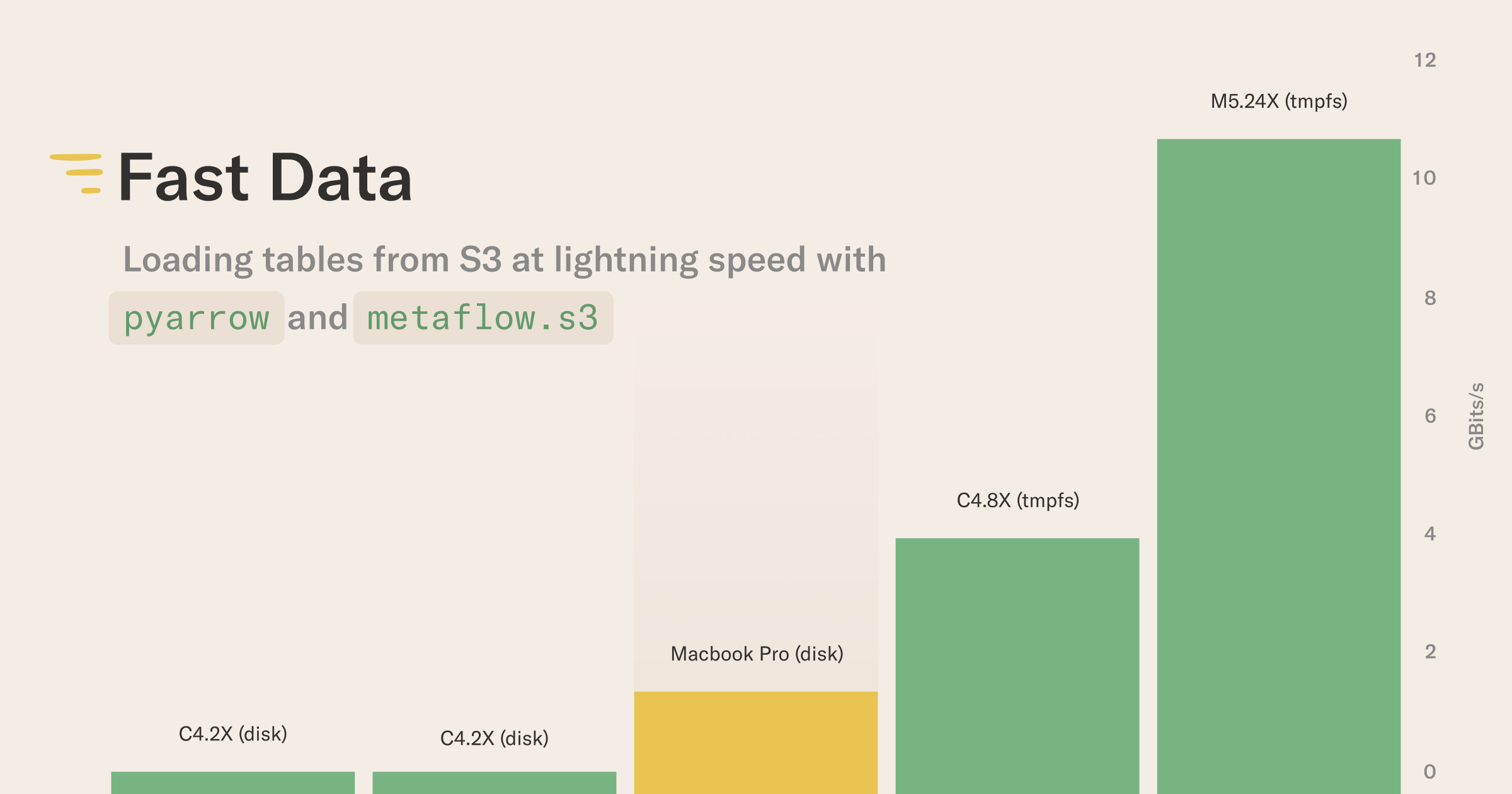
This article answers a common question: How can I load tabular data quickly from S3 into a Metaflow workflow and process it efficiently? Thanks to Metaflow’s straightforward support for vertical scalability, its high-throughput S3 client, and high-performance tooling powered by Apache Arrow, you can handle surprisingly large amounts of data, surprisingly fast.
You can execute all benchmarks and examples with the code in this repository.
Ever since the early days of Metaflow at Netflix, we have been asking a fundamental question from data scientists and other users of Metaflow: What is the greatest source of friction in your day to day work? Maybe unsurprisingly, the majority of answers relate to data: Finding the right data, accessing data, transforming data, and utilizing data in various ways.
In contrast to traditional software, which has a limited surface area with the outside world, data exposes ML/AI-powered applications to constantly changing real-world entropy and complexity. It would be unreasonable to expect that we can address the diverse use cases with a single nifty solution. Needs differ greatly, say, between computer vision, NLP, large tabular data, and small datasets.
We can support a wide variety of use cases by working well with a broad set of open-source data tools and efficient infrastructure. This approach is illustrated by our view of the full stack of ML infrastructure which acknowledges the need of providing plenty of support for data:
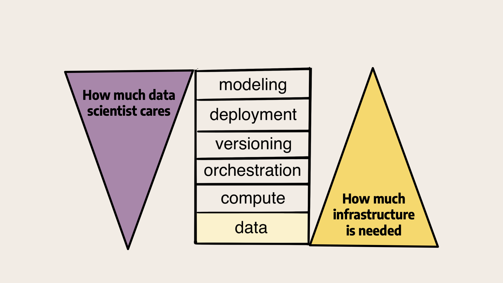
Metaflow doesn’t provide magical new abstractions or paradigms for processing data, but it provides foundational, human-friendly infrastructure that works smoothly with the tools of your choice. Data scientists certainly care about data but data tooling should just work without hassle. Often simpler is better.
This article focuses on a common use case of data: tabular, structured datasets. This use case is particularly interesting, as tooling for it has evolved rapidly over the past few years.
A fast path for tabular data
All modern data warehousing solutions either store data natively as Parquet-encoded files (like various versions of the cloud-based data lake e.g. powered by AWS Athena or Spark), or they allow exporting/unloading data as Parquet files (e.g. Snowflake or Redshift).
Conveniently, these systems allow you to create materialized views which can be processed outside the warehouse. You can use SQL and the Create-Table-As-Select (CTAS) pattern to query even petabytes of data, extracting the results for downstream processing in Metaflow.
Once you have Parquet files in S3, you can hit the fast path:
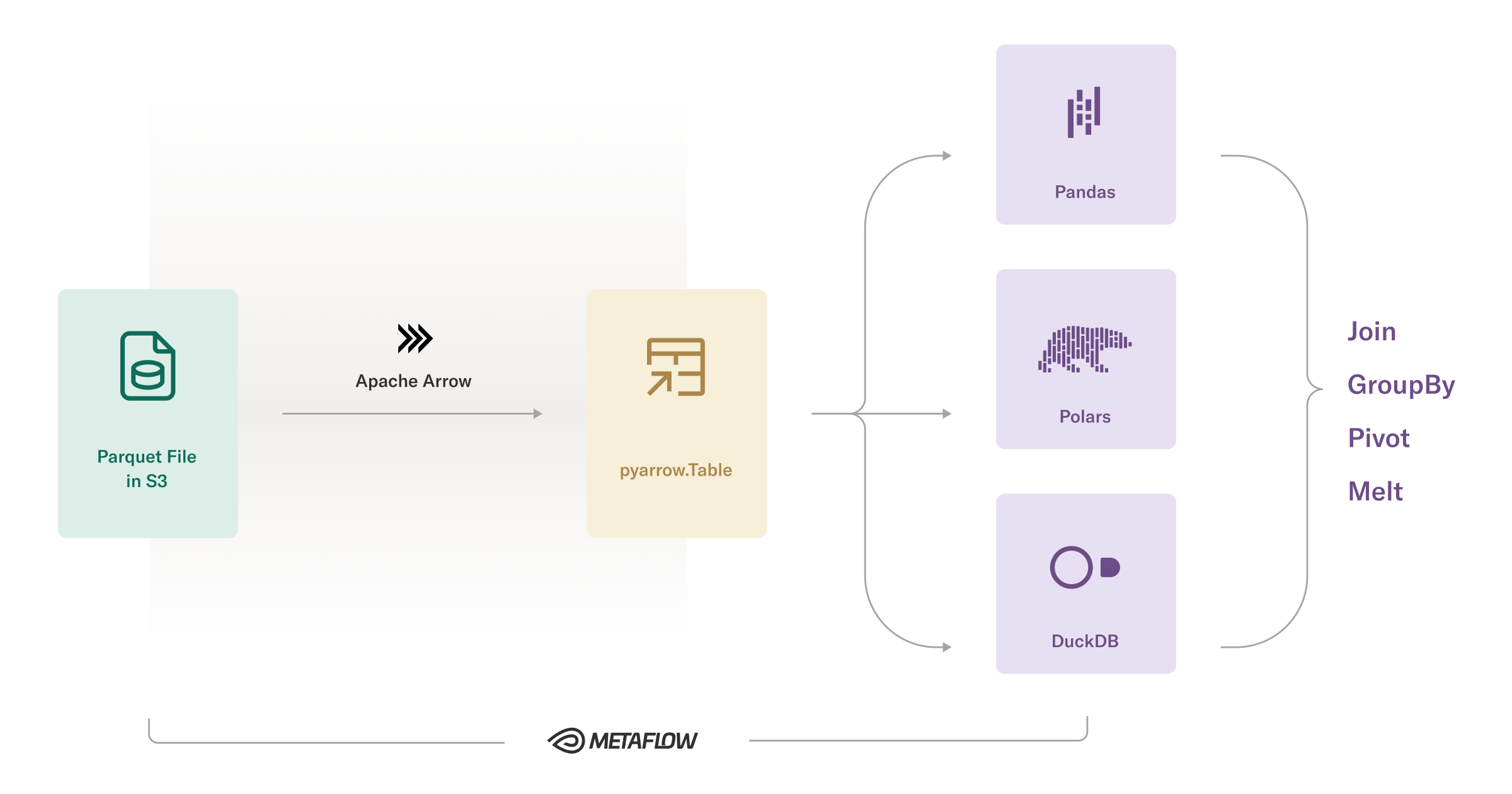
You can load data from S3 directly to memory very quickly, at tens of gigabits per second or more, using Metaflow’s optimized S3 client,
metaflow.S3.Once in memory, Parquet data can be decoded efficiently using Apache Arrow.
The in-memory tables produced by Arrow are interoperable with various modern data tools, so you can use the data in various ways without making additional copies, which speeds up processing and avoids unnecessary memory overhead.
This pattern is becoming increasingly popular, thanks to the maturation of Apache Arrow itself and versatile tools around it. The excitement is further motivated by the realization that a single medium-size EC2 instance can handle an amount of data that used to require a Hadoop or Spark cluster just a decade ago - this time with much fewer operational headaches, and at a much lower cost.
The pattern is still new, so not everyone is fully aware of how well and fast it works - under suitable conditions. To showcase this, we first focus on the left side of the diagram, addressing a common myth that loading data from S3 is slow. After this, we focus on the right side, demonstrating how to use the data with various high-performance tools efficiently.
S3 is fast (when used correctly)
Occasionally, we are asked how to cache data from S3 on local disk, instance volume, or a distributed file system like EFS to make loading and processing data faster. Counterintuitively, loading data from S3 can be much faster than local disk, so there's no need to add extra layers of complexity.
The question likely stems from first-hand experiences of S3 being slow, which can easily happen if you don’t have a setup that leverages its strengths. This benchmark illustrates the point:
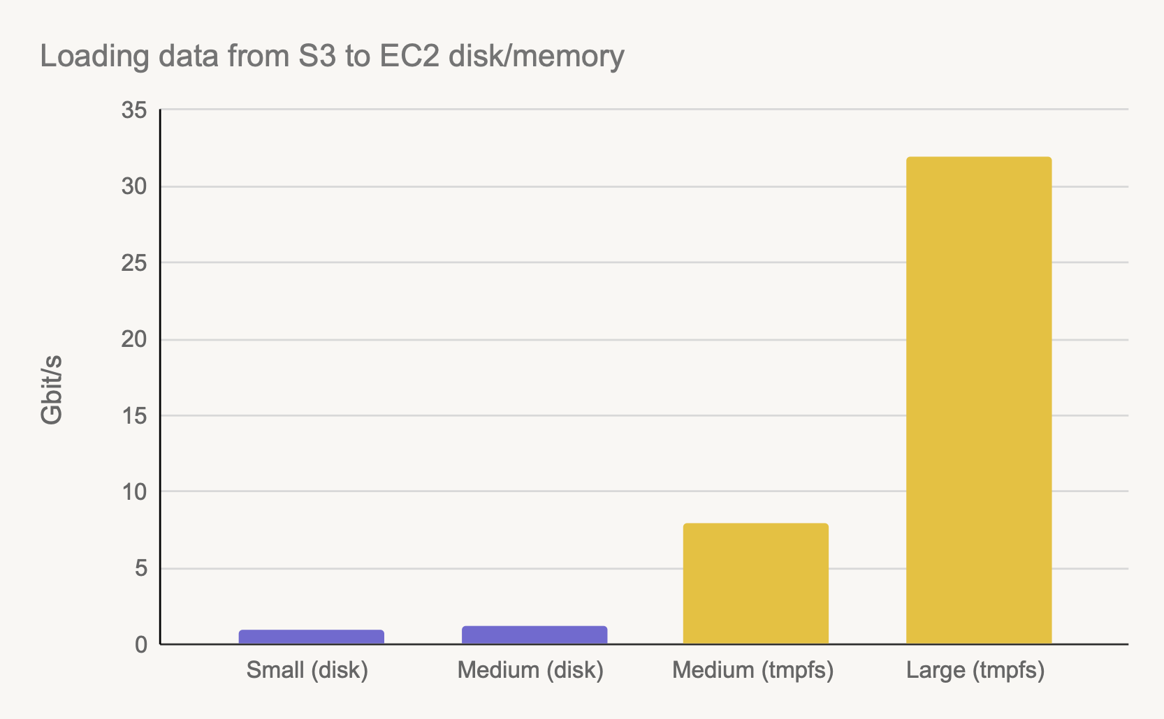
The bars refer to a Metaflow task that uses metaflow.S3 to download the dataset, running on EC2 with AWS Batch using the @batch decorator, comparing four different configurations:
- Small (disk): 8GB RAM, 2 CPU cores, a c4.2xlarge instance with EBS.
- Medium (disk): 8GB RAM, 8 CPU cores, a c4.8xlarge instance with EBS.
- Medium (tmpfs): 30GB RAM, 8 CPU cores, a c4.8xlarge utilizing Metaflow’s new
tmpfsfeature. - Large (tmpfs): 200GB RAM, 32 CPU cores, an m5n.24xlarge utilizing Metaflow’s new
tmpfsfeature.
There is a 35x fold speed difference between the slowest and the fastest configuration! Understandably, if your tasks ran under the first configuration, you would conclude that S3 is slow.
Maximizing the S3 performance
A key observation is that the download throughput of S3 is a combination of multiple factors. In order to achieve the maximum throughput, pay attention to the following dimensions:
- Same region: Make sure the EC2 instances hosting the tasks are located in the same region as the S3 bucket you are loading data from.
- File layout: You need to download multiple files in parallel using e.g. metaflow.S3.get_many. The files should be around 0.1-1GB each. Fortunately, it is easy to produce partitioned outputs like this with many query engines.
- Instance size: Larger EC2 instances boost higher number of CPU cores, network throughput, and memory. When using e.g.
@batchwith Metaflow, instances autoscale based on demand, so faster processing times can lead to lower costs, despite the higher unit costs of larger instances. - Data fits in RAM: Crucially, loading data from S3 directly to memory is faster than loading data from S3 to an instance volume. If data doesn’t fit in memory, performance can be very bad due to slow local disk IO.
The importance of the last point is demonstrated by the two medium bars: By increasing the amount of memory available for the tasks - simply by setting @resources(memory=32000) - we gain an eightfold increase in S3 throughput!
The highest bar demonstrated the massive horsepower available on the largest instances: By using metaflow.S3, we can reach a beast-mode throughput of 32 GBit/s, which can easily beat local SSDs on laptops. In other words, loading data from S3 to an EC2 instance can be faster than loading data locally on a laptop, or loading it from an EBS volume, an ephemeral instance disk, or EFS.
New feature: tmpfs support for Batch and Kubernetes
We have been using the above fast data pattern successfully for years to power Metaflow workflows handling terabytes of data. However, this far, there has been a small gotcha.
While allocating enough memory through @resources should guarantee that data can be downloaded quickly, we still rely on the local filesystem to back the files nominally, although the files never hit the disk thanks to caching. Sadly, it is not possible to allocate disk space for tasks on the fly while using AWS Batch. Doing it requires a bit more tedious change in the instance’s launch template.
To address this issue, recently we implemented support for memory-based tmpfs filesystem on Batch and Kubernetes in Metaflow. You can use the feature to create an ephemeral filesystem backed by memory on the fly, without having to change anything on the infrastructure side.
We made sure that the metaflow.S3 client is aware of the tmpfs volume, so it will automatically use it to speed up downloads when you enable it. To benefit from the new feature, simply add
@batch(use_tmpfs=True)
for your AWS Batch workloads or
@kubernetes(use_tmpfs=True)
for Kubernetes. There are a few additional features related to tmpfs which you can read more about in the Metaflow documentation.
From cloud to table
As shown above, we can load bytes to memory very quickly. To actually use the data, we must also decode the Parquet files to an in-memory pyarrow.Table object. When taking the decoding time into account, the differences are even more striking:
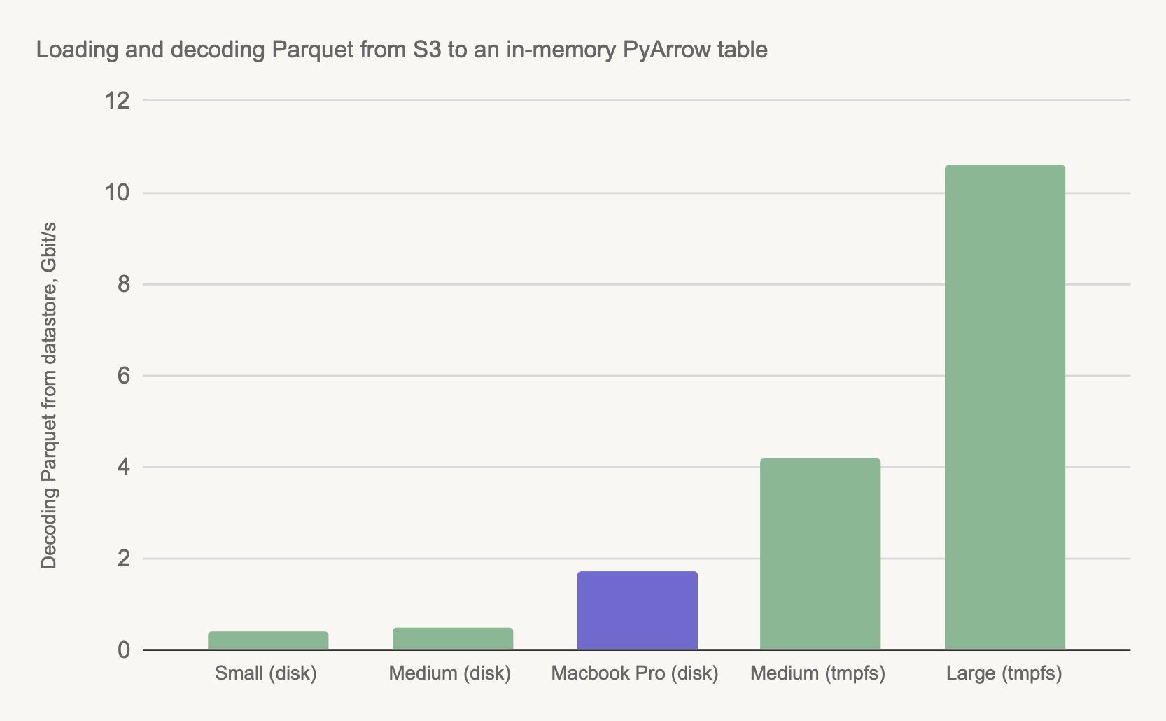
The configurations are the same as in the first chart above. We added a top-of-the-line M2 Macbook Pro (the purple bar) as a comparison point. The Macbook loads data from a local SSD, not from S3 as the instances do.
As shown above, a powerful Macbook beats small and medium-size instances when the instances are using a local disk, but even a medium-size instance beats the Macbook when using in-memory processing. In this case, a large instance can load a table about 8x faster than a Macbook.
This result is a combination of multiple factors: The larger instances have more CPU cores, more memory, and more IO bandwidth available than a Macbook. Naturally, you must utilize the resources efficiently to gain the maximum performance: Use metaflow.S3.get_many to maximize network throughput and multithreaded decoding to benefit from all the available CPU cores, as exemplified by the table_loader.py utility module.
From table to results
With a pyarrow.Table object in memory, the possibilities are many! We highlight three common use cases below.
Crucially, all the libraries listed below support zero-copy instantiation from a pyarrow.Table, so you don’t have to reserve a large amount of extra @resources(memory=) just to handle extra copies or inefficient internal representations. Ballooning memory overhead used to be a problem in the past with older Pandas, prior to Arrow.
You can code along with the following sections using this repository.
Dataframes
Moving to Pandas is trivial and fast:
df = table.to_pandas()
You can add a zero_copy_only=True flag to make sure that you will get warned if the conversion requires extra copies of data. Since the Pandas 2.0 release that came out just a month ago, Pandas is fully compatible with Arrow data types, so working with Arrow and Pandas should be smooth sailing.
While Pandas provides a familiar API, its operations are not always the fastest. You can often enjoy a higher performance by using Polars - a high-performance dataframe library:
import polars as pl
df = pl.from_arrow(table)
SQL
Sometimes it is more convenient to use SQL for data processing than dataframe APIs. For instance, you can follow this pattern to enable clear division of responsibilities between data engineers and data scientists:
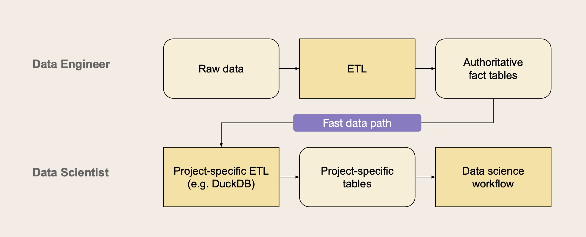
In this scenario, data engineers are responsible for maintaining company-wide, authoritative fact tables that individual projects can rely on. Projects may create their own interpretations of data through their own lightweight ETL process e.g. for feature transformations.
The project-specific ETL can run within their Metaflow workflows using a small but surprisingly powerful in-process database, DuckDB. A benefit of this approach is that data scientists can own and iterate on their specific ETL very quickly, even testing it locally on their workstations.
Using this pattern is not harder than using a dataframe:
import duckdb
query = "SELECT * FROM arrow_table"
relation = duckdb.arrow(arrow_table)
df = relation.query('arrow_table', query).to_df()
To familiarize with using DuckDB and Metaflow together in a machine learning context, you can follow along with this recommender systems tutorial.
Interfacing with ML libraries
Many modern ML libraries are well optimized when it comes to utilizing CPU and GPU resources. However, to benefit from high-performance training and inferencing, you need to be able to feed data to the model fast.
Luckily, Arrow data is readily convertible to Pandas and NumPy which are supported by all major ML libraries. Through NumPy, you can also convert data to various tensor objects.
To illustrate the pattern, we included a simple ML example that shows how to convert an Arrow table to a Pandas dataframe, and feed this object to a LightGBM model. The flow trains a model to predict a target variable based on 300 finance instruments.
You can run the code easily by yourself and visualize the results through a Metaflow card, like this one:
Summary
This post outlined patterns that you can use to load tabular data from S3 to your Metaflow workflows quickly and process it in various ways using Arrow-compatible libraries.
In future posts, we will dive deeper into related topics around data: How to use data engineering tools like dbt together with Metaflow, how to handle large datasets in a horizontally scalable manner using the patterns highlighted here, and how to make sure that the pattern comply with your data governance policies.
You can test patterns highlighted here in the Metaflow sandbox. If you have any feedback, questions, or other thoughts around data, join us and thousands of other data scientists and engineers on Metaflow Slack!
PS. If open-source data topics pique your interest, join our upcoming event on The Open-Source Modern Data Stack on June 7th.


