Scale to the clouds

A key benefit of Outerbounds is its ease of accessing scalable compute resources. You can

• scale vertically by utilizing large cloud instances,
• scale horizontally by executing even thousands of tasks in parallel,
• access powerful GPUs,
• and spin up clusters of (GPU) instances on the fly for distributed computing.

Or, you can leverage any combination of these approaches to suit your needs.

Scaling up and out

As an example, imagine that you want to train a model which needs at least 16B of memory and 2 CPU cores to finish quickly. To make the case more interesting, imagine that you want to train a separate model for a number of countries, say USA, Canada, Brazil, and China, in parallel.

The ScalableFlow shows how to implement the idea (you can replace the dummy code in train with a real trainer, if you like). It uses two key constructs for scalability, highlighted in the code:

• foreach spawns a separate task for each item in the list of countries to express parallelism.

• @resources is used to request compute resources - here, 2 CPU cores and 16GB of RAM for each training task.

After training four models in parallel, the join step receives all the models via the inputs argument and chooses the best performing model, storing it in an artifact, best.

import random
from metaflow import FlowSpec, step, resources

class ScalableFlow(FlowSpec):

    @step
    def start(self):
        self.countries = ['US', 'CA', 'BR', 'CN']
        self.next(self.train, foreach='countries')

    @resources(cpu=2, memory=16000)
    @step
    def train(self):
        print('training model...')
        self.score = random.randint(0, 10)
        self.country = self.input
        self.next(self.join)

    @step
    def join(self, inputs):
        self.best = max(inputs, key=lambda x: x.score).country
        self.next(self.end)

    @step
    def end(self):
        print(self.best, 'produced best results')

if __name__ == '__main__':
    ScalableFlow()

Save the flow in a file, scaleflow.py. You could execute it locally as python scaleflow.py run - Metaflow makes it easy to test code locally before scaling to the cloud - but to benefit from additional compute @resources and parallelism, use run --with kubernetes:

python scaleflow.py run --with kubernetes

The flow may take a while to start, as new cloud instances may need to be brought up to handle the workload. You can monitor the run in the Runs view as usual.

---

This is all you have to know to start scaling up and out with Outerbounds. Take a look at the next article about defining execution environments to address a few practical issues with real-like projects.

If you want to learn how the scalable cluster works under the hood, keep on reading.

Observing the cluster status

Behind the scenes, Outerbounds spins up new cloud instances automatically to execute your workload. If you are curious to know how the cluster is behaving, you can open the Status view which shows the cluster status and configuration in detail.

The chart on the left shows the total demand for compute resources, aggregated over all running tasks. If the demand exceeds 100% of the currently available compute resources, indicated by the red line, the cluster auto-scales to bring more instances online.

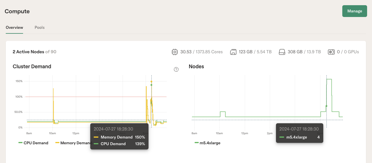
The chart on the right illustrates the number of instances online. You can observe that the number increases shortly after the spike in the left chart and decreases once the tasks are completed. This auto-scaling behavior makes Outerbounds cost-efficient, as you only pay for the instances when they are actively needed.

What kind of compute resources can I request?

The available resources depend on your cluster configuration. You can check the currently available Compute pools by clicking the Pools tab in the Status view.

If you try to request resources that are not available, you will get an error message. For instance, you can try to request an instance with 512GB of RAM to be used for all steps in a flow:

python scaleflow.py run --with kubernetes:memory=512000

In the likely scenario that you don't have instances with 512GB of RAM configured, you will see an error message and the flow refuses to execute.

Configuring compute pools

Outerbounds allows you to federate compute pools from various sources. You can use

• any cloud instances in your primary cloud account,
• any cloud instances form other clouds, combining resources from AWS, Azure, and GCP,
• GPU resources from NVIDIA's private DGX cloud,
• or you can even use on-prem resources as a part of the unified cluster.

Contact your dedicated Slack channel to request any changes in the compute pool.