Using cost reports
This page explains how to utilize the three cost reports available in the Cost Reports section. These reports assist you in understanding and optimizing your compute costs. Before exploring the details, we recommend reviewing the Overview of cost optimization.
Historical cost
The Historical Spend view shows an estimate of compute costs incurred by the platform over the past 30 days:
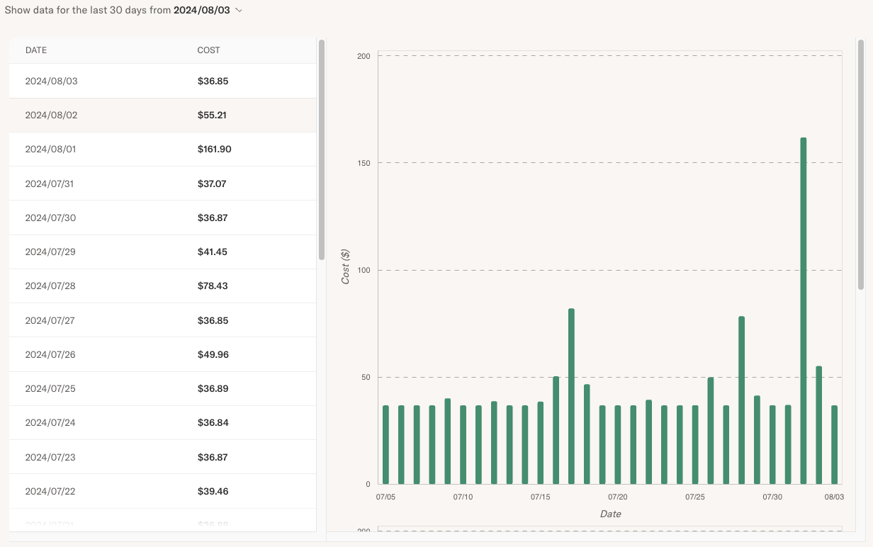
The purpose of this view is to provide a quick overview of whether costs are within the expected range and to indicate if further optimizations are needed. If the cost is within an acceptable range, you don't have to do anything else!
The view updates daily. You can choose an earlier 30-day time range in the dropdown in the top left corner.
Note the following about the cost estimate:
The dollar amounts are based on the cloud's list pricing, not your negotiated pricing. The amounts don't include any discounts e.g. through reserved instances. Hence, your actual compute costs are likely to be lower.
The amounts indicate the variable cost component driven by compute on the platform. They don't indicate the total cost of the platform which includes data storage and database costs. However, the data costs are typically small compared to compute costs and they grow only slowly with respect to the amount of workloads.
Currently, all amounts are quoted in dollars, even if your account is set to use another currency.
In contrast to many other platforms, Outerbounds doesn't charge extra margin on compute. The prices reflected on this view are the list prices quoted by each cloud.
Instance usage
To gain a detailed understanding of the daily costs shown in the historical view, open the Node Report, which displays the instances used on a given day. For example, in the historical screenshot above, you can observe a cost spike on August 1st. Drilling down into that day can help us understand why the costs were higher than expected.
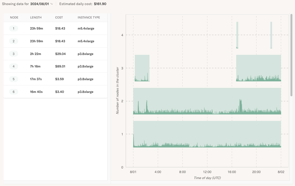
On the right, you can see a 24-hour timeline with all instances that ran on that day overlaid on it. The legend on the left shows the instance type and the associated cost incurred by each instance. The total of these instance costs matches the amount shown in the historical view.
The chart inside each instance span on the timeline shows the utilization of the instance.
With a quick glance, we can see that a large cost driver was a p3.8xlarge instance
running for 7 hours on that day, costing $89.
Why was an instance provisioned
A natural follow-up question is why the instance was provisioned. Click on a span or an item in the list to open a more detailed view that shows the flows and steps assigned to the instance.
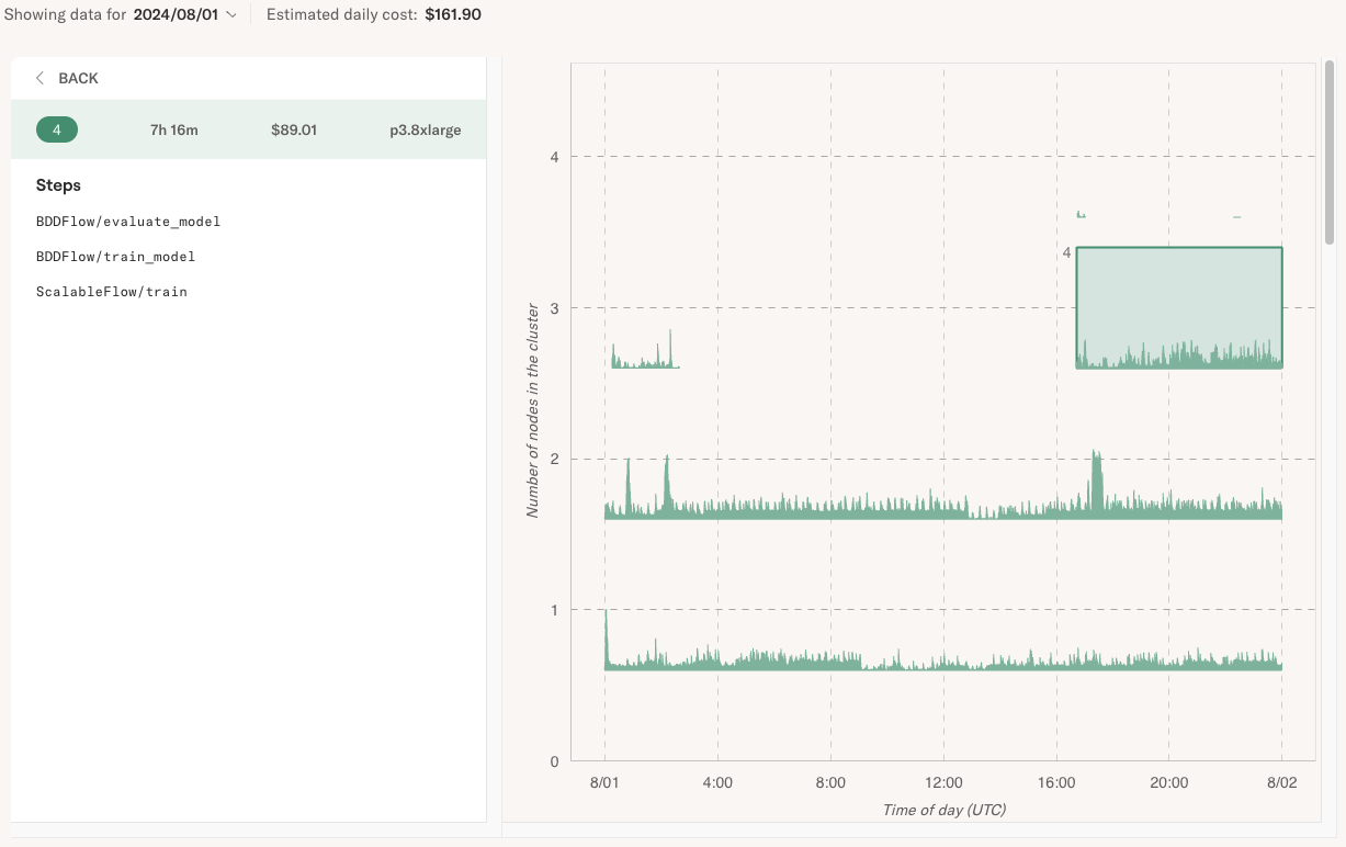
You can see that in this case BODFlow training and evaluation, as well as ScalableFlow
were running on the instance.
Resource utilization
To understand if tasks are using resources they request efficiently, open the Flow Report. This view provides a treasure trove of information about workloads.
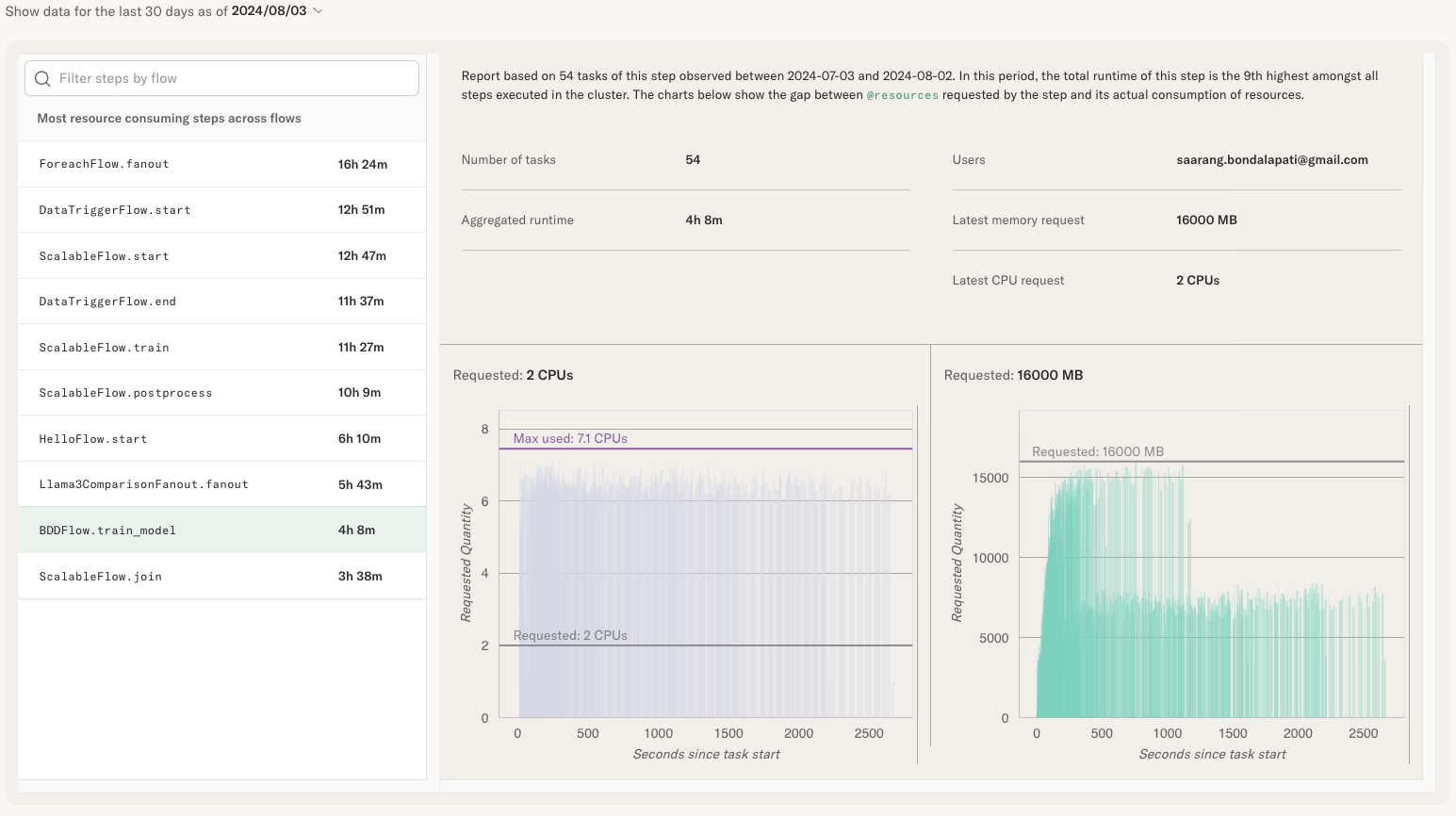
The list on the left is ordered by the total amount of instance hours consumed by a step.
Typically, the top items on the list are the highest cost drivers and hence a natural target
for optimization. You can also choose a certain step, like BODFlow.train_model that we
saw running on an expensive node on August 1st earlier.
On the right, you can see charts showing resource utilization of the selected step. Note the following about the charts:
The purple chart on the left shows CPU utilization and the green chart on the right memory utilization.
The X axis on the chart shows seconds since the task started. Often a task may exhibit bespoke behavior during its lifetime, e.g. a higher memory consumption after data has been loaded in memory.
The charts aggregate resource consumption of the selected step over the past 30 days. Hence you see multiple time series overlaid in the chart, giving you an idea of the overall behavior while also revealing outliers.
A gray horizontal bar shows the amount of CPU or memory requested through the
@resourcesdecorator. A purple bar showing the maximum resources used is shown if it differs from the resources requested.
For instance, in the above screenshot, the step requested 2 CPU cores but actually spiked to
over 7 CPU cores. It might be prudent to increase the CPU resources to @resources(cpu=7)
to ensure sufficient resources for the task. We can also observe that the task utilized
the 16GB of requested memory efficiently, though memory consumption drops during the second half
of the task's execution.
Observing resource utilization in real time
The cost reporting views are focused on aggregating information over a longer period of time, updating daily. Typically, you don't want to optimize resource requirements based on a single datapoint, especially if the task consumes changing data which may affect its behavior over time.
However, during development it is useful to see if the resource requirements are in the right ballback. You can see resource usage in real-time in the task view, under Task graphs:
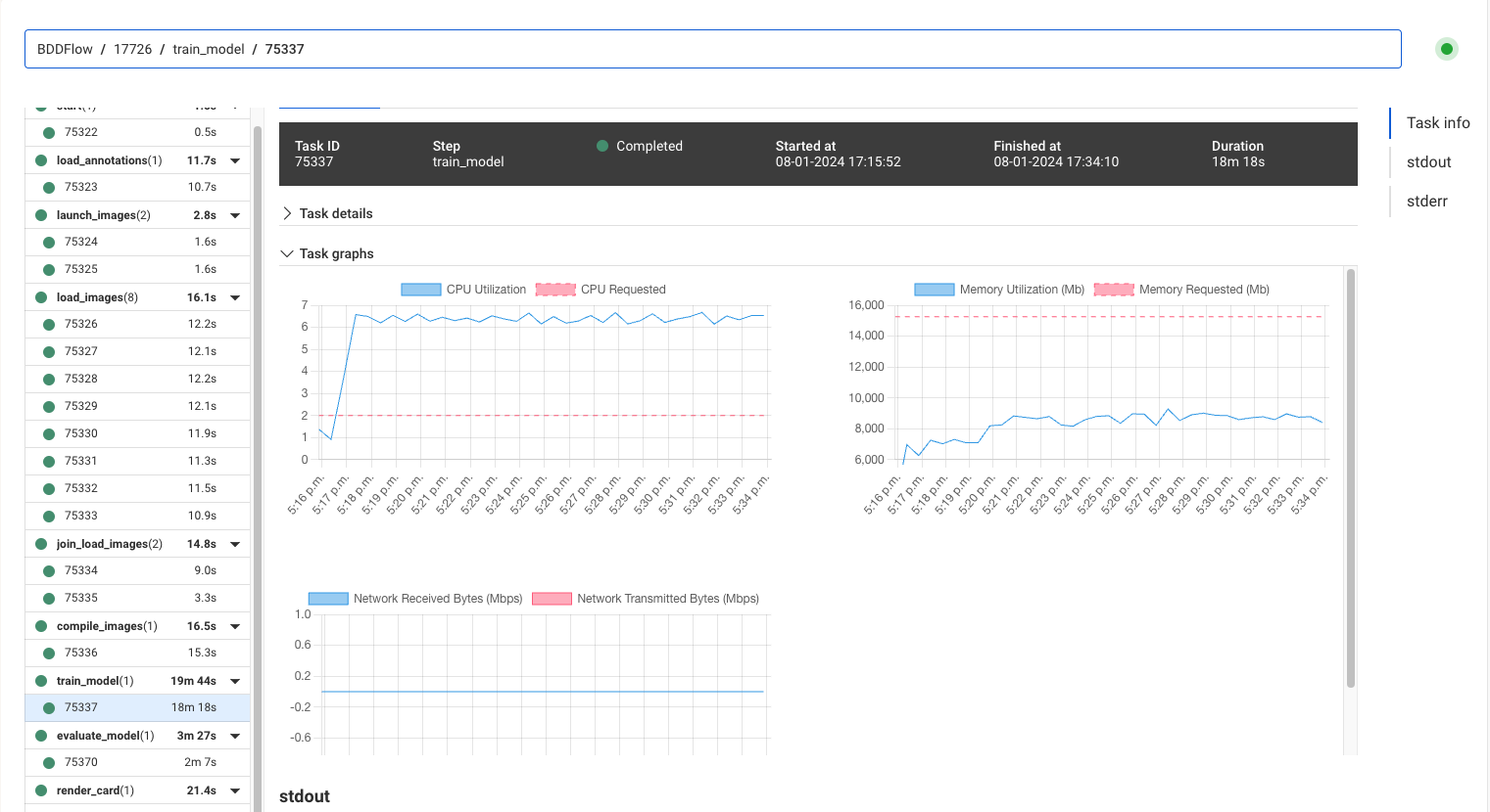
Currently task graphs are only available for tasks that execute for longer than a minute.
Looking at one of the BODFlow.train_model tasks, we can see that the CPU utilization is hovering
at around 7 CPU cores (the blue line), while the requested amount (the red line) is 2 CPU cores,
which aligns with the numbers shown in the aggregated cost reports.
Looking at memory consumption of this particular task, which hovers at around 9GB, we might underestimate the true memory requirements across tasks, which sometimes peak at 16GB as shown in the aggregated cost report.
A downside of setting @resources too low, especially for memory, is that the task may crash due
to an Out-Of-Memory error, which is generally worse than slight underutilization of resources.
Identifying resource underutilization
This example highlights a case of resource underutilization:
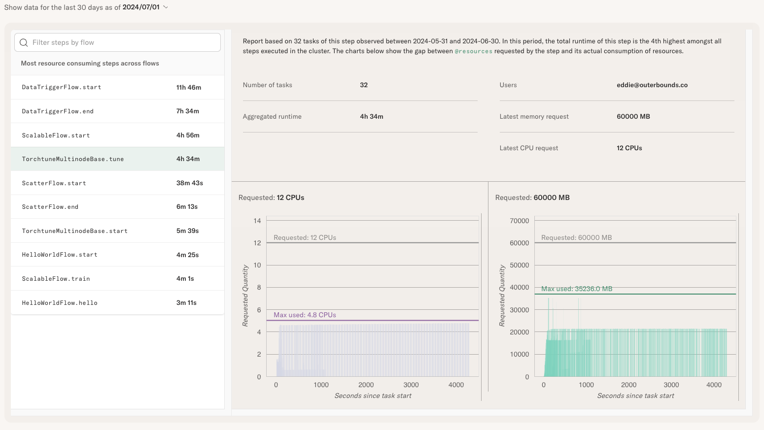
The task requests 12 CPU cores but never uses more than 5 CPU cores. Similarly, it requests 60GB
of memory but peaks at 35GB of memory used. In this case, you could right-size @resources to
@resources(cpu=5, memory=36000) without having an adverse effect on the task. This frees up
resources on the instance, allowing other tasks to be scheduled on the instance simultaneously,
increasing utilization and lowering the total compute costs.
@resources automatically?Given this information, you might wonder if the system could right-size @resources automatically?
A challenge is that the resource consumption is typically a function of input data which might
grow or shrink over time. As of today, we rely on your understanding of the data and use cases to
adjust the resources if needed.