// File: custom-components-preview ## CardStack ### Usage ```
), }} />
), }} />
``` ### Output
), }} />
), }} />
## OpenSandbox ### Usage ``` We highly recommend [taking a backup of your RDS instance](https://docs.aws.amazon.com/AmazonRDS/latest/UserGuide/CHAP_CommonTasks.BackupRestore.html) before attempting this upgrade. This will allow you to restore the service from the backup in case there are any issues with the migration. ``` ### Output We highly recommend [taking a backup of your RDS instance](https://docs.aws.amazon.com/AmazonRDS/latest/UserGuide/CHAP_CommonTasks.BackupRestore.html) before attempting this upgrade. This will allow you to restore the service from the backup in case there are any issues with the migration. ## TutorialSandbox ### Usage ``` ``` ### Output ## CustomAdmonition ### Usage ``` Build workflows to train and evaluate a real world model that performs image classification using Keras. ``` ### Output Build workflows to train and evaluate a real world model that performs image classification using Keras. We highly recommend [taking a backup of your RDS instance](https://docs.aws.amazon.com/AmazonRDS/latest/UserGuide/CHAP_CommonTasks.BackupRestore.html) before attempting this upgrade. This will allow you to restore the service from the backup in case there are any issues with the migration. ## RHS Components Group of components to render right-hand side content which is connected to the main pane content. ### RHS Component to render right-hand side content. When the right-hand side content is placed in the `Wrapper` component, it's aligned to the other content present in the `Wrapper` component. Otherwise, it'll be using a `fixed` position on the right side of the screen. ### Wrapper Helper component to define the position of right-hand side content. ### Highlight Helper component to drive attention to right-hand side content. ### Usage ```` This flow leverages the functions in `torch_steps.py` to: * Create dataloaders for training and testing. * Train multiple models in parallel on GPU instances using Metaflow's `@batch` decorator in the `train` step. The example uses Metaflow's `@conda` decorator to create a similar environment across local and remote compute. ```py title="scale_tuning_gpu.py" from metaflow import (FlowSpec, step, Parameter, batch, JSONType, conda_base) import json import torch_steps ``` Lorem ipsum dolor sit amet, consectetur adipiscing elit, sed do eiusmod tempor incididunt ut labore et dolore magna aliqua. Ut enim ad minim veniam, quis nostrud exercitation ullamco laboris nisi ut aliquip ex ea commodo consequat. ```` ### Output This flow leverages the functions in `torch_steps.py` to: - Create dataloaders for training and testing. - Train multiple models in parallel on GPU instances using Metaflow's `@batch` decorator in the `train` step. The example uses Metaflow's `@conda` decorator to create a similar environment across local and remote compute. ```py title="scale_tuning_gpu.py" from metaflow import (FlowSpec, step, Parameter, batch, JSONType, conda_base) import json import torch_steps ``` Lorem ipsum dolor sit amet, consectetur adipiscing elit, sed do eiusmod tempor incididunt ut labore et dolore magna aliqua. Ut enim ad minim veniam, quis nostrud exercitation ullamco laboris nisi ut aliquip ex ea commodo consequat. ## NumberHeading Adds a number next to the heading. | Prop | Type | Description | | -------- | ------ | ------------------------------------------ | | children | string | Text to be shown | | number | number | Number to be displayed next to the heading | ### Usage ``` ## Heading level 2 ### Heading level 3 #### Heading level 4 ``` ### Output ## Heading level 2 ### Heading level 3 #### Heading level 4 ## CustomCode Allows to either limit the height of a code block or make it collapse by default. | Prop | Type | Description | | ----------- | ---------- | ---------------------------------------------------------------- | | height | string | Height of the code block to be consumed by CSS `height` property | | collapse | boolean | Tells the component either it should be `details` or `div` | | sandboxLink | string | link to sandbox | | children | code block | Text to be shown | ### Usage ```` ```py title="wandb_helpers.py" import os import wandb def plot_results(X_train, y_train, X_test, y_test, y_pred, y_probs, clf, labels): wandb.init(entity=os.getenv("WANDB_ENTITY"), project=os.getenv("WANDB_PROJECT"), mode="offline") wandb.sklearn.plot_class_proportions(y_train, y_test, labels) wandb.sklearn.plot_learning_curve(clf, X_train, y_train) wandb.sklearn.plot_roc(y_test, y_probs, labels) wandb.sklearn.plot_precision_recall(y_test, y_probs, labels) wandb.sklearn.plot_feature_importances(clf) wandb.sklearn.plot_classifier( clf, X_train, X_test, y_train, y_test, y_pred, y_probs, labels, is_binary=True, model_name='RandomForest' ) wandb.finish() ``` ```` ### Output ```py title="wandb_helpers.py" import os import wandb def plot_results(X_train, y_train, X_test, y_test, y_pred, y_probs, clf, labels): wandb.init(entity=os.getenv("WANDB_ENTITY"), project=os.getenv("WANDB_PROJECT"), mode="offline") wandb.sklearn.plot_class_proportions(y_train, y_test, labels) wandb.sklearn.plot_learning_curve(clf, X_train, y_train) wandb.sklearn.plot_roc(y_test, y_probs, labels) wandb.sklearn.plot_precision_recall(y_test, y_probs, labels) wandb.sklearn.plot_feature_importances(clf) wandb.sklearn.plot_classifier( clf, X_train, X_test, y_train, y_test, y_pred, y_probs, labels, is_binary=True, model_name='RandomForest' ) wandb.finish() ``` ## Caption Adds a caption to be used underneath an image | Prop | Type | Description | | -------- | ------ | ---------------- | | children | string | Text to be shown | ### Usage ``` Image Description ``` ### Output Image Description ## CodeOutputBlock | Prop | Type | Description | | -------- | -------------------- | ----------------------- | | children | code block or string | Output code to be shown | ### Usage ``` Workflow starting (run-id 1647826193209570): [1647826193209570/start/1 (pid 8372)] Task is starting. [1647826193209570/start/1 (pid 8372)] Task finished successfully. [1647826193209570/middle/2 (pid 8375)] Task is starting. [1647826193209570/middle/2 (pid 8375)] Task finished successfully. [1647826193209570/end/3 (pid 8378)] Task is starting. [1647826193209570/end/3 (pid 8378)] Task finished successfully. Done! ``` ### Output Workflow starting (run-id 1647826193209570): [1647826193209570/start/1 (pid 8372)] Task is starting. [1647826193209570/start/1 (pid 8372)] Task finished successfully. [1647826193209570/middle/2 (pid 8375)] Task is starting. [1647826193209570/middle/2 (pid 8375)] Task finished successfully. [1647826193209570/end/3 (pid 8378)] Task is starting. [1647826193209570/end/3 (pid 8378)] Task finished successfully. Done! ## PageDescription Shows a description of a page | Prop | Type | Description | | -------- | ------ | ---------------- | | children | string | Text to be shown | ### Usage ``` Image Description ``` ### Output Description of the page ## DocLink Show a button with a link to a document with an icon | Prop | Type | Description | | -------- | ------ | ------------------- | | link | url | Document to link to | | children | string | Label for the link | ### Usage ``` Notebook documents ``` ### Output Notebook documents ## DocSection Renders JSX that comes from docstrings in Python code to show API documentation more clearly. ### Usage ``` ``` ### Output ### Description | Prop | Type | Description | | | ---------------- | ---- | ----------------------------- | -------- | | extended_summary | md | Further description text | optional | | summary | md | First line of the description | required | ### DocSection | Prop | Type | Description | | | ------------- | ------------------- | -------------------------------------------- | -------- | | baseUrl | url | Base URL for the source link | optional | | children | Component[] | Components for each section of the docstring | required | | heading_level | number | Heading level at which to show the name | optional | | module | string | The module that contains the code | optional | | name | string | The name of the code being described | required | | type | "class" or "method" | The type of code being described | optional | ### Parameter | Prop | Type | Description | | | ---- | ------ | ---------------------------- | -------- | | desc | md | Description of the parameter | optional | | name | string | Name of the parameter | required | | type | md | Type of the parameter | optional | ### ParamSection | Prop | Type | Description | | | ---- | ------ | ------------------- | -------- | | name | string | Name of the section | required | ### SigArg | Prop | Type | Description | | | ---- | ------ | ---------------------------- | -------- | | name | string | Name of a signature argument | required | ### SigArgSection | Prop | Type | Description | | | -------- | -------- | ---------------------------- | -------- | | children | SigArg[] | Components for each argument | required | ## HTMLOutputBlock Renders HTML within MDX. Used for complex output that includes HTML and javascript. | Prop | Type | Description | | -------- | ---------- | --------------------------------------- | | center | boolean | If true, center the output horizontally | | children | code block | HTML to be shown | ### Usage ``` Countdown: let count = 999999; setInterval(()=>\{ count -=1; const el = document.getElementById("count_example"); debugger; if (el) \{ el.innerHTML = count; } }, 1000); Countdown: ## Login Widget ``` ``` --- // File: data-science/compute/build_custom_image ## Question How can I build a custom docker image to run a Metaflow step? ## Solution Metaflow has decorators to run steps on remote compute environments like `@batch` and `@kubernetes`. The environments these jobs run in can both be created from a Docker image. In some circumstances you may need to create your own image for running a step or a flow. In this case there are a few things to consider when building your image. #### Specify an Image in a Flow First it is important to mention how Metaflow knows which image to use. You can read more about using a custom image [here](/use-custom-image). If you do not specify the image argument like `@batch(image="my_image:latest")`, Metaflow will look to see if you have [configured](/engineering/operations/configure-metaflow/) a default container image for the compute plugin you are using in the `METAFLOW_DEFAULT_CONTAINER_IMAGE` variable. If this configuration is not specified and you do not specify the `image` argument in the decorator, the image is built from the [official Python image](https://hub.docker.com/_/python/) for the version of Python you are using in your local environment. ### Write a Dockerfile Docker images are built using a Dockerfile. When building one to use with Metaflow there are a few considerations to keep in mind. #### Base Image A minimum requirement is that you will need Python in the image - we suggest starting from an official Python image. For example, you can add the following at the start of your Dockerfile: ``` FROM python:3.10 ``` The image should come with standard CLI tools like tar, so we suggest avoiding starting the Dockerfile with `FROM scratch`. #### User Permissions Metaflow needs to be able to write in the working directory. In the Dockerfile this concerns the `WORKDIR` and `USER` commands. You should make sure that the user running commands can write in the working directory, especially when you do explicitly set these in your Dockerfile. Note that many images use root user by default, and Metaflow does not so you may have to explicitly specify a non-root `USER` in your Dockerfile. You can use the following to check the user for your image: ```bash docker run --rm -it bash -c id ``` For example, by default this Python image user id is root: ```bash docker run --rm -it python:3.10 bash -c id ``` ``` uid=0(root) gid=0(root) groups=0(root) ``` You can change the user in the Dockerfile like ```Dockerfile FROM my_base_image:latest USER my_user ... ``` #### Using ENTRYPOINT and CMD We suggest you do not set either of these in your Dockerfile. Metaflow [constructs a command](https://github.com/Netflix/metaflow/blob/62f5e52ebce755d9130287c1576011cb056e0e3d/metaflow/metaflow_environment.py#L83-L102) to run the container for you, so defining the ENTRYPOINT too can produce unexpected errors. #### Example Here is an example of a standard Dockerfile. * The `WORKDIR` is changed and the `USER` has write permission. * The `COPY` command moves a `requirements.txt` file into the image and installs the contents. You could follow a similar copying process to install custom modules that are not on PyPi. * Also notice there is no CMD or ENTRYPOINT since Metaflow will override this for you anyways. ```Dockerfile title="Dockerfile" FROM python:3.10 RUN mkdir /logs && chown 1000 /logs RUN mkdir /metaflow && chown 1000 /metaflow ENV HOME=/metaflow WORKDIR /metaflow USER 1000 COPY requirements.txt requirements.txt RUN pip install --no-cache-dir --upgrade pip && \ pip install --no-cache-dir -r requirements.txt ``` ### Build your Image This process is not unique to Metaflow. Once you have written a Dockerfile like the one above, you can [build it](https://docs.docker.com/engine/reference/commandline/build/) from the directory like: ```bash docker build . ``` If you are building or running your image on MacOS, and plan to later deploy to a Linux machine, you will need to specify `--platform=linux/amd64` in your build and run commands. For example, when using the EC2 instances that power AWS Batch environments you will want to make sure the image is built for the right platform. You can set the platform automatically when building and running images by using an environment variable: ``` export DOCKER_DEFAULT_PLATFORM=linux/amd64 ``` Another alternative is to specify the platform in the beginning of your Dockerfile: ``` FROM --platform=linux/amd64 image:tag ``` ### Configure Metaflow to Use your Image Once you have built your image you need to tell Metaflow to use it. This requires pushing the image to a registry that you have permission to access. For example, in AWS you might want your image to reside in [ECR](https://docs.aws.amazon.com/AmazonECR/latest/userguide/docker-push-ecr-image.html). In a flow the most direct way to tell Metaflow to use this image for a step is to use the plugin decorators like `@batch(image=:)` and `@kubernetes(image=:)`. You can also set default environment variables so Metaflow knows to look for a certain image in a specified container registry by default. Some configuration variables to keep in mind for specifying a URI for a default image and container registry are `METAFLOW_DEFAULT_CONTAINER_IMAGE` and `METAFLOW_DEFAULT_CONTAINER_REGISTRY`. * `METAFLOW_DEFAULT_CONTAINER_IMAGE` dictates the default container image that Metaflow should use. * `METAFLOW_DEFAULT_CONTAINER_REGISTRY` controls which registry Metaflow uses to pick the image - this defaults to DockerHub. These will then be used as a default across compute plugins. [Metaflow configuration variables](/engineering/operations/configure-metaflow/) can be set in the active `METAFLOW_PROFILE` stored in `~/.metaflow-config/` or as environment variables. For example, if your container registry is in AWS ECR you can set an environment variable like: ```bash export METAFLOW_DEFAULT_CONTAINER_REGISTRY=.dkr.ecr..amazonaws.com ``` and then decorate your flow steps like: ```python @batch(image="image-in-my-registry:latest") @step def containerized_step(self): ... ``` Alternatively, you can specify the registry, image, and tag all in the decorator: ```python @batch(image="url-to-docker-repo/docker-image:version") @step def containerized_step(self): ... ``` Note that if you are manually configuring the underlying resources for remote compute plugins (as opposed to automating deployment through CloudFormation or Terraform) you will need to make ensure that the appropriate roles are available for those resources. ## Further Reading * [Use a custom image](/use-custom-image) in your flow * See configuration details in: [metaflow_config.py](https://github.com/Netflix/metaflow/blob/493d406347c11787d73f0cc76fb798d8526b4955/metaflow/metaflow_config.py) * See where in the Metaflow code image and container registry variables are used for [@batch](https://github.com/Netflix/metaflow/blob/master/metaflow/plugins/aws/batch/batch_decorator.py#L112-L138) and [@kubernetes](https://github.com/Netflix/metaflow/blob/master/metaflow/plugins/kubernetes/kubernetes_decorator.py#L101-L121) * [Building a Dockerfile for a Python environment](https://docs.docker.com/language/python/build-images/) * [Understand how CMD and ENTRYPOINT interact](https://docs.docker.com/engine/reference/builder/#understand-how-cmd-and-entrypoint-interact) * [Best practices for containerizing Python applications with Docker](https://snyk.io/blog/best-practices-containerizing-python-docker/) --- // File: data-science/compute/package_files_for_remote_compute ## Question How do I package files so they are usable in remote compute steps? ## Solution Metaflow includes all `.py` files in your flow script's directory in the distribution. This means all `.py` file dependencies will be available in remote compute environments. The rest of this page shows how to include files that do not end in `.py` using the `--package-suffixes` argument. :::note This page describes how to use the `--package-suffixes` command line argument. You can also use the `METAFLOW_DEFAULT_PACKAGE_SUFFIXES` configuration option. ::: ### Define a Dependency in the Flow Directory Suppose you have the following two `.sql` files in your flow script's directory and you want to access them on a remote compute instance. ```sql title="query1.sql" SELECT * FROM DB1; ``` ```sql title="query2.sql" SELECT * FROM DB2; ``` :::note This pattern is not unique to the `.sql` file extension. ::: ### Define a Flow that Uses the Dependencies Remotely This flow shows how to: * Run the `start` step remotely using Kubernetes. * Use the `query1.sql` and `query2.sql` files in the remote compute environment. ```py title="package_suffixes_flow.py" from metaflow import FlowSpec, step, kubernetes class PackageSuffixesFlow(FlowSpec): query1_file = 'query1.sql' query2_file = 'query2.sql' def read_query(self, file): file_obj = open(file, 'r') result = file_obj.read() file_obj.close() return result @kubernetes @step def start(self): self.query1 = self.read_query(self.query1_file) self.query2 = self.read_query(self.query2_file) self.next(self.end) @step def end(self): print("Query 1:", self.query1) print("Query 2:", self.query2) if __name__ == "__main__": PackageSuffixesFlow() ``` ### Package the Dependencies and Run the Flow The key to this page is Metaflow's `package-suffixes` argument. To run the `PackageSuffixesFlow` and copy the local `.sql` files so they are accessible in the `start` step running in a Kubernetes pod, you can run the following command: ```bash python package_suffixes_flow.py --package-suffixes='.sql' run ``` ``` Workflow starting (run-id 186474): [186474/start/1009082 (pid 67155)] Task is starting. [186474/start/1009082 (pid 67155)] [pod t-8dvdn-8f2mw] Task is starting (Pod is pending, Container is waiting - ContainerCreating)... [186474/start/1009082 (pid 67155)] [pod t-8dvdn-8f2mw] Setting up task environment. [186474/start/1009082 (pid 67155)] [pod t-8dvdn-8f2mw] Downloading code package... [186474/start/1009082 (pid 67155)] [pod t-8dvdn-8f2mw] Code package downloaded. [186474/start/1009082 (pid 67155)] [pod t-8dvdn-8f2mw] Task is starting. [186474/start/1009082 (pid 67155)] [pod t-8dvdn-8f2mw] Task finished with exit code 0. [186474/start/1009082 (pid 67155)] Task finished successfully. [186474/end/1009083 (pid 67159)] Task is starting. [186474/end/1009083 (pid 67159)] Query 1: SELECT * FROM DB1; [186474/end/1009083 (pid 67159)] [186474/end/1009083 (pid 67159)] Query 2: SELECT * FROM DB2; [186474/end/1009083 (pid 67159)] [186474/end/1009083 (pid 67159)] Task finished successfully. Done! ``` ## Further Reading * [Load Local Data with IncludeFile](/load-local-data-with-include) * [Share Local Data with S3 in Metaflow](/sharing-local-data-with-s3) --- // File: data-science/compute/scale_tuning_on_gpu ## Question How do I scale model training and hyperparameter tuning to GPUs with Metaflow? ## Solution To scale horizontally, you can structure Metaflow flows with branching and looping patterns. To scale vertically you can access more processor and memory resources for a task in your flow by using Metaflow's `@batch` and `@kubernetes` decorators. ### Define PyTorch Dependencies This example will show how to tune a PyTorch model on GPUs. The script contains functions to * Load data. * Instantiate a neural net. * Train and evaluate a neural net. The [original code](https://pytorch.org/tutorials/beginner/blitz/cifar10_tutorial.html#training-an-image-classifier) for the example comes from the PyTorch documentation. ```py title="torch_steps.py" import torch import torchvision import torch.optim as optim import torchvision.transforms as transforms import torch.nn as nn import torch.nn.functional as F class Net(nn.Module): def __init__(self): super().__init__() self.conv1 = nn.Conv2d(3, 6, 5) self.pool = nn.MaxPool2d(2, 2) self.conv2 = nn.Conv2d(6, 16, 5) self.fc1 = nn.Linear(16 * 5 * 5, 120) self.fc2 = nn.Linear(120, 84) self.fc3 = nn.Linear(84, 10) def forward(self, x): x = self.pool(F.relu(self.conv1(x))) x = self.pool(F.relu(self.conv2(x))) # flatten all dims except batch x = torch.flatten(x, 1) x = F.relu(self.fc1(x)) x = F.relu(self.fc2(x)) x = self.fc3(x) return x def load_data(): transform = transforms.Compose( [transforms.ToTensor(), transforms.Normalize((0.5, 0.5, 0.5), (0.5, 0.5, 0.5))]) batch_size = 4 trainset = torchvision.datasets.CIFAR10( root='./data', train=True, download=True, transform=transform ) trainloader = torch.utils.data.DataLoader( trainset, batch_size=batch_size, shuffle=True, num_workers=2 ) testset = torchvision.datasets.CIFAR10( root='./data', train=False, download=True, transform=transform ) testloader = torch.utils.data.DataLoader( testset, batch_size=batch_size, shuffle=False, num_workers=2 ) classes = ('plane', 'car', 'bird', 'cat','deer', 'dog', 'frog', 'horse', 'ship', 'truck') return trainloader, testloader, classes def train_model(trainloader, lr, epochs=1): net = Net() if torch.cuda.is_available(): device = torch.device('cuda:0') else: device = torch.device('cpu') net.to(device) criterion = nn.CrossEntropyLoss() optimizer = optim.SGD(net.parameters(), lr=lr, momentum=0.9) for epoch in range(epochs): for i, data in enumerate(trainloader, 0): inputs = data[0].to(device) labels = data[1].to(device) optimizer.zero_grad() outputs = net(inputs) loss = criterion(outputs, labels) loss.backward() optimizer.step() return net def run_inference_and_tests(net, testloader): correct = 0 total = 0 with torch.no_grad(): for data in testloader: images, labels = data outputs = net(images) _, predicted = torch.max(outputs.data, 1) total += labels.size(0) correct += (predicted == labels).sum().item() return 100 * correct // total ``` ### Run Flow This flow leverages the functions in `torch_steps.py` to: * Create dataloaders for training and testing. * Train multiple models in parallel on GPU instances using Metaflow's `@batch` decorator in the `train` step. * In this case each model will get a different learning rate assigned. This is simple for demo purposes, in practice you will want to explore more dimensions of hyperparameter space when you have the resources. * Evaluate each model. * Join the results of evaluation to select the best model. * Print the highest accuracy model. * You can improve the model by changing hyperparameters in `torch_steps.py` or by expanding the hyperparameter tuning task with more branches in the flow. The example uses Metaflow's `@conda` decorator to create a similar environment across local and remote compute. ```py title="scale_tuning_gpu.py" from metaflow import (FlowSpec, step, Parameter, batch, JSONType, conda_base) import json import torch_steps @conda_base(libraries={"pytorch":"1.11.0", "torchvision":"0.12.0"}, python="3.8") class GPUFlow(FlowSpec): learning_rates = Parameter( 'learning-rates', default=json.dumps([0.01,0.001]), type=JSONType ) @step def start(self): data = torch_steps.load_data() self.trainloader = data[0] self.testloader = data[1] self.classes = data[2] self.next(self.train, foreach='learning_rates') @batch(gpu=1) @step def train(self): self.model = torch_steps.train_model( self.trainloader, lr=self.input ) self.next(self.evaluate_model) @step def evaluate_model(self): result = torch_steps.run_inference_and_tests( self.model, self.testloader ) self.accuracy = result self.next(self.join) @step def join(self, inputs): best_model = None; best_score = -1 for i in inputs: if i.accuracy > best_score: best_score = i.accuracy best_model = i.model self.best_model = best_model self.best_score = best_score print(f"Best model accuracy was {best_score}%.") self.next(self.end) @step def end(self): print("Done") if __name__ == "__main__": GPUFlow() ``` ```bash python scale_tuning_gpu.py --environment=conda run ``` ``` ... [560/start/2899 (pid 65768)] Task is starting. [560/start/2899 (pid 65768)] Downloading https://www.cs.toronto.edu/~kriz/cifar-10-python.tar.gz to ./data/cifar-10-python.tar.gz 100.0%05-24 21:25:42.845 [560/start/2899 (pid 65768)] 0.0%9%4.2% [560/start/2899 (pid 65768)] Extracting ./data/cifar-10-python.tar.gz to ./data [560/start/2899 (pid 65768)] Files already downloaded and verified [560/start/2899 (pid 65768)] Foreach yields 2 child steps. [560/start/2899 (pid 65768)] Task finished successfully. ... [560/join/2904 (pid 65886)] Task is starting. [560/join/2904 (pid 65886)] Best model accuracy was 46%. [560/join/2904 (pid 65886)] Task finished successfully. ... [560/end/2905 (pid 65898)] Task is starting. [560/end/2905 (pid 65898)] Done [560/end/2905 (pid 65898)] Task finished successfully. ... ``` ## Further Reading * [How to use multiple CPU cores inside of Metaflow tasks](/use-multiple-cpu-cores) * [Scale out and up](https://docs.metaflow.org/v/r/metaflow/scaling) * [PyTorch distributed overview](https://pytorch.org/tutorials/beginner/dist_overview.html) --- // File: data-science/compute/use_custom_image ## Question How can I use a custom docker image to run a Metaflow step? ## Solution Metaflow has decorators to run steps on remote compute environments like `@batch` and `@kubernetes`. The environments run jobs created from a Docker image. ### Select an Image You can either [build an image](/build-custom-image) or choose one. If you choose an existing image, make sure that Python can be invoked from the container. You can tell Metaflow which image you want to use in several ways: * passing the `image` argument in a decorator like `@batch(image="my_image:latest")` * in [Metaflow config files](/engineering/operations/configure-metaflow/) * `METAFLOW_DEFAULT_CONTAINER_REGISTRY` controls which registry Metaflow uses to pick the image - this defaults to DockerHub but could also be a URL to a public or private ECR repository on AWS. * `METAFLOW_DEFAULT_CONTAINER_IMAGE` dictates the default container image that Metaflow should use. * don't specify and let Metaflow default to the [official Python image](https://hub.docker.com/_/python/) * in this case, the default corresponds to the major.minor version of Python that the user used to launch the flow ### Run Flow For example, this flow uses the [official Python image](https://hub.docker.com/_/python/) in the `run_in_container` step. In this example only the image name and tag is specified but know that you can also pass in the full URL to the image in `@batch` or `@kubernetes` - `@batch(image="url-to-docker-repo/docker-image:version")`. #### Note about GPU images In these decorators you will see resource arguments like `cpu=1`. Assuming that your Metaflow deployment allows you to access compute instances with GPU resources, you can also set `gpu=N` and Metaflow will automatically prepare your image in a way that works with GPU. In this example access means that the AWS Batch compute environment will need access to [EC2 instances with GPUs](https://aws.amazon.com/ec2/instance-types/#Accelerated_Computing). ```py title="use_image_flow.py" from metaflow import FlowSpec, step, batch, conda import os class UseImageFlow(FlowSpec): @step def start(self): self.next(self.run_in_container) #highlight-next-line @batch(image="python:3.10", cpu=1) @step def run_in_container(self): self.artifact_from_container = 7 self.next(self.end) @step def end(self): pass if __name__ == "__main__": UseImageFlow() ``` ```bash python use_image_flow.py run ``` ``` Workflow starting (run-id 685): [685/start/3463 (pid 33227)] Task is starting. [685/start/3463 (pid 33227)] Task finished successfully. [685/run_in_container/3464 (pid 33231)] Task is starting. [685/run_in_container/3464 (pid 33231)] [98f8111b-76f1-4e04-97d4-7d7bc2c58abd] Task is starting (status SUBMITTED)... [685/run_in_container/3464 (pid 33231)] [98f8111b-76f1-4e04-97d4-7d7bc2c58abd] Task is starting (status STARTING)... [685/run_in_container/3464 (pid 33231)] [98f8111b-76f1-4e04-97d4-7d7bc2c58abd] Task is starting (status RUNNING)... [685/run_in_container/3464 (pid 33231)] [98f8111b-76f1-4e04-97d4-7d7bc2c58abd] Setting up task environment. [685/run_in_container/3464 (pid 33231)] [98f8111b-76f1-4e04-97d4-7d7bc2c58abd] Downloading code package... [685/run_in_container/3464 (pid 33231)] [98f8111b-76f1-4e04-97d4-7d7bc2c58abd] Code package downloaded. [685/run_in_container/3464 (pid 33231)] [98f8111b-76f1-4e04-97d4-7d7bc2c58abd] Task is starting. [685/run_in_container/3464 (pid 33231)] [98f8111b-76f1-4e04-97d4-7d7bc2c58abd] Task finished with exit code 0. [685/run_in_container/3464 (pid 33231)] Task finished successfully. [685/end/3465 (pid 33245)] Task is starting. [685/end/3465 (pid 33245)] Task finished successfully. Done! ``` ### Access Artifacts Outside of Flow The following can be run in a Python script or notebook to access the artifact produced in the container step: ```python from metaflow import Flow run = Flow("UseImageFlow").latest_run assert run.successful # get data produced in containerized step artifact = run.data.artifact_from_container assert artifact == 7 ``` ## Further Reading * [Build a custom image](/build-custom-image) * Set environment variables in a container using [Metaflow's @environment decorator](/set-env-vars-with-decorator) or [.env file](/set-env-vars-with-file) * See where in the Metaflow code image and container registry variables are used for [@batch](https://github.com/Netflix/metaflow/blob/master/metaflow/plugins/aws/batch/batch_decorator.py#L112-L138) and [@kubernetes](https://github.com/Netflix/metaflow/blob/master/metaflow/plugins/kubernetes/kubernetes_decorator.py#L101-L121) --- // File: data-science/compute/use_multiple_cpu_cores ## Question How can I use multiple CPU cores within Metaflow tasks? ## Answer You can use multiple cores like you normally would in your Python code in a Metaflow task. For example, you can use Python's [concurrent.future](https://docs.python.org/3/library/concurrent.futures.html) module to launch multiple processes and threads. ### Write Flow with Concurrency in a Task This flow shows how to: - Call the `do_task` function four times on different cores using Python's built-in `concurrent.futures.ThreadPoolExecutor`. - Print the total time elapsed to demonstrate the tasks ran in parallel. ```py title="use_multiple_cpu_cores.py" from metaflow import FlowSpec, step, Parameter from concurrent import futures import time def do_task(name): time.sleep(3) # a long-running task return name class MulticoreFlow(FlowSpec): #highlight-next-line num_cores = Parameter('num-cores', default=4) @step def start(self): threads = [ "thread_%s" % i for i in range(self.num_cores) ] t0 = time.time() #highlight-start with futures.ThreadPoolExecutor( max_workers = self.num_cores ) as exe: self.messages = [ msg for msg in exe.map(do_task, threads) ] #highlight-end self.time_elapsed = time.time() - t0 self.next(self.end) @step def end(self): print_msg = "All tasks completed in %.3fs" print(print_msg % self.time_elapsed) [print(msg) for msg in self.messages] if __name__ == '__main__': MulticoreFlow() ``` ### Run Flow ```bash python use_multiple_cpu_cores.py run ``` ``` Workflow starting (run-id 1663278003721691): [1663278003721691/start/1 (pid 47937)] Task is starting. [1663278003721691/start/1 (pid 47937)] Task finished successfully. [1663278003721691/end/2 (pid 47941)] Task is starting. [1663278003721691/end/2 (pid 47941)] All tasks completed in 3.011s [1663278003721691/end/2 (pid 47941)] thread_0 [1663278003721691/end/2 (pid 47941)] thread_1 [1663278003721691/end/2 (pid 47941)] thread_2 [1663278003721691/end/2 (pid 47941)] thread_3 [1663278003721691/end/2 (pid 47941)] Task finished successfully. Done! ``` ## Further Reading * [Parallelization Over Multiple Cores](https://docs.metaflow.org/metaflow/scaling-out-and-up/effortless-scaling-with-kubernetes#parallelization-over-multiple-cores) * [How to Scale Model Training and Tuning to GPU](/scale-model-training-and-tuning/) --- // File: data-science/data/chunk-dataframe ## Question I have a large pandas dataframe in memory. How can I chunk it into Parquet files using Metaflow? ## Solution You can do this using Metaflow's foreach. A pattern you can use to do this is to use Apache Arrow's zero copy slice ability with Metaflow's foreach. ### Gather data Suppose you have curated a dataset: ```python import numpy as np import pandas as pd import string from datetime import datetime letters = list(string.ascii_lowercase) make_str = lambda n: ''.join(np.random.choice(letters, size=n)) dates = pd.date_range(start=datetime(2010,1,1), end=datetime.today(), freq="min") size = len(dates) df = pd.DataFrame({ 'date': dates, 'num1': np.random.rand(size), 'num2': np.random.rand(size), 'str1': [make_str(20) for _ in range(size)], 'str2': [make_str(20) for _ in range(size)] }) df.to_csv("./large_dataframe.csv") ``` ```python df.head(3) ``` ```html
date num1 num2 str1 str2
0 2010-01-01 00:00:00 0.424410 0.503014 xyouzjaivrwtnqczcieb fonxhwjxdpdvnfvtvcar
1 2010-01-01 00:01:00 0.650159 0.184204 dxrqtbmezgwobpqlpybt ihahasnbtgptjfwnvlic
2 2010-01-01 00:02:00 0.602216 0.647338 kaatnygdfekoxmpnvbky wffzxlyzjnopahttvdxe
```
and your goal is to store this data efficiently in Parquet files. ### Determine How to Chunk the Data [Pyarrow](https://arrow.apache.org/docs/python/generated/pyarrow.Table.html) version `5.0.0` is used to split the dataframe into chunks. You can see how in this utility function that will be used in the following flow: ```py title="dataframe_utils.py" import pyarrow as pa import pandas as pd from datetime import datetime from typing import List, Tuple def get_chunks(df:pd.DataFrame = None, num_chunks:int = 4) -> Tuple[pa.Table, List]: get_year = lambda x: datetime.strptime( x.split()[0], "%Y-%m-%d").year df['year'] = df.date.apply(get_year) num_records = df.shape[0] // num_chunks lengths = [num_records] * num_chunks lengths[-1] += df.shape[0] - num_chunks*num_records offsets = [sum(lengths[:i]) for i in range(num_chunks)] names = ["chunk_%s" %i for i in range(num_chunks)] return (pa.Table.from_pandas(df), list(zip(names, offsets, lengths))) ``` ### Run Flow This flow shows how to load this into a pandas dataframe and apply the following steps: * Use `pyarrow.from_pandas` method to load the data to Arrow memory. * In parallel branches: * Use `pyarrow.Table.slice` to make zero-copy views of chunks of the table. * Apply a transformation to the table; appending a column in this case * Move the chunks to your S3 bucket using `pyarrow.parquet.write_table`. * Pick a chunk and verify the existence of the new transformed column. If you have a dataframe in S3 that you want to read into memory, you can see an example specific to this topic [here](/load-parquet-data-to-pandas-df). ```py title="chunk_dataframe.py" from metaflow import FlowSpec, step class ForEachChunkFlow(FlowSpec): bucket = "s3://outerbounds-how-tos" s3_path = "{}/dataframe-chunks/{}.parquet" df_path = "./large_dataframe.csv" @step def start(self): import pandas as pd from dataframe_utils import get_chunks my_big_df = pd.read_csv(self.df_path) self.table, self.chunks = get_chunks(my_big_df) self.next(self.process_chunk, foreach='chunks') @step def process_chunk(self): import pyarrow as pa import pyarrow.parquet as pq # get view of this chunk only chunk_id, offset, length = self.input chunk = self.table.slice(offset=offset, length=length) # do transformation on table col1 = chunk['num1'].to_numpy() col2 = chunk['num2'].to_numpy() values = pa.array(col1 * col2) chunk = chunk.append_column('new col', values) # write chunk as parquet file in S3 bucket self.my_path = self.s3_path.format(self.bucket, chunk_id) pq.write_table(table=chunk, where=self.my_path) self.next(self.join) @step def join(self, inputs): self.next(self.end) @step def end(self): import pyarrow.parquet as pq test_id = 'chunk_1' path = self.s3_path.format(self.bucket, test_id) test_chunk = pq.read_table(source=path) assert 'new col' in test_chunk.column_names if __name__ == "__main__": ForEachChunkFlow() ``` ```bash python chunk_dataframe.py run ``` ``` Workflow starting (run-id 1658839758360594): [1658839758360594/start/1 (pid 65431)] Task is starting. [1658839758360594/start/1 (pid 65431)] Foreach yields 4 child steps. [1658839758360594/start/1 (pid 65431)] Task finished successfully. [1658839758360594/process_chunk/2 (pid 65447)] Task is starting. [1658839758360594/process_chunk/3 (pid 65448)] Task is starting. [1658839758360594/process_chunk/4 (pid 65449)] Task is starting. [1658839758360594/process_chunk/5 (pid 65450)] Task is starting. [1658839758360594/process_chunk/5 (pid 65450)] Task finished successfully. [1658839758360594/process_chunk/4 (pid 65449)] Task finished successfully. [1658839758360594/process_chunk/2 (pid 65447)] Task finished successfully. [1658839758360594/process_chunk/3 (pid 65448)] Task finished successfully. [1658839758360594/join/6 (pid 65592)] Task is starting. [1658839758360594/join/6 (pid 65592)] Task finished successfully. [1658839758360594/end/7 (pid 65595)] Task is starting. [1658839758360594/end/7 (pid 65595)] Task finished successfully. Done! ``` ## Further Reading * [Loading and Storing Data in Metaflow](https://docs.metaflow.org/metaflow/data#data-in-local-files) * [Load Parquet Data from S3 to Arrow Table](/load-parquet-data-to-arrow-table) --- // File: data-science/data/fast-cloud-to-table ## Question I have a set of `.parquet` files in the cloud, and want to read them into memory on my remote workers quickly. How can I do this with Metaflow? ## Solution 1. You can load data from S3 directly to memory very quickly, at tens of gigabits per second or more, using Metaflow’s optimized S3 client, metaflow.S3. 2. Once in memory, Parquet data can be decoded efficiently using Apache Arrow. 3. The in-memory tables produced by Arrow are interoperable with various modern data tools, so you can use the data in various ways without making additional copies, which speeds up processing and avoids unnecessary memory overhead. ### Cloud to table Before writing a Metaflow flow, let's see how to use the [Metaflow S3 client](https://docs.metaflow.org/scaling/data) with [Apache Arrow](https://arrow.apache.org/). The main steps to pay attention to are that we use the [`metaflow.S3.get_many` function](https://docs.metaflow.org/api/S3#S3.get_many) to parallelize the retrieval of partitions of the `.parquet` file, loading the bytes into memory on the worker instance, and decoding the bytes so they are useful in a `pyarrow.Table` object. ```python from metaflow import S3 import pyarrow.parquet as pq import pyarrow from concurrent.futures import ThreadPoolExecutor import multiprocessing ``` ```python # Instantiate Metaflow S3 client context s3 = S3() # Set the URL of an S3 bucket containing .parquet files url = "s3://outerbounds-datasets/ubiquant/investment_ids" ``` To check metadata about what exists in the S3 url of interest without actually downloading the files, you can use [`metaflow.s3.list_recursive`](https://docs.metaflow.org/scaling/data#listing-objects-in-s3). ```python files = list(s3.list_recursive([url])) total_size = sum(f.size for f in files) / 1024**3 print("Loading%2.1dGB of data partitioned across %d files." % (total_size, len(files))) ``` ``` Loading 7GB of data partitioned across 3579 files. ``` ```python # Download the files in parallel loaded = s3.get_many([f.url for f in files]) ``` Notice the loaded files are in temporary storage in `./metaflow.s3.foobar`. ```python print(len(loaded)) print(loaded[0]) print(loaded[0].path) ``` ``` 3579 ./metaflow.s3.v_cz59co/9946232270752e97d9247ed2907154d2ea0b8841-0_parquet-whole ``` ```python local_tmp_file_paths = [f.path for f in loaded] ``` In another set of parallel processes, read the PyArrow tables from bytes and then concatenate them. :::tip The benefits of this workflow scale with the number of processors, available RAM, and I/O throughput of the machine you are loading a table on. Bigger instances can be cheaper in many cases, since they can reduce processing times at a super-linear rate. More on this later in the post. ::: ```python with ThreadPoolExecutor(max_workers = multiprocessing.cpu_count()) as exe: tables = exe.map(lambda f: pq.read_table(f, use_threads=False), local_tmp_file_paths) table = pyarrow.concat_tables(tables) ``` ```python print("Table has %d rows and%2.1dGB bytes in memory." % (table.shape[0], table.nbytes / 1024**3)) ``` ``` Table has 3141410 rows and 7GB bytes in memory. ``` ```python # close s3 connection s3.close() ``` ### Performance benefits scale with instance size Using the basic pattern described above, you can now write Metaflow flows that scale this fast data speedup on cloud instances. In this workflow, we organize the same operations presented in section 1 in a Metaflow flow. Notice that the `data_processing` step is annotated with `@batch(..., use_tmpfs=True, ...)`. The `tmpfs` feature extends the resources you request, because it allows you to use memory on the Batch instance to instantiate a temporary file system; this makes the cloud-to-table workflow significantly faster and does not require using the local file system to temporarily store the `.parquet` bytes. To reiterate, the benefits of this workflow scale with the number of processors, available RAM, and I/O throughput of the machine you are loading a table on; so you will want to use an instance that can fit your entire Arrow table in memory to get maximal benefits. To get a sense of how fast this workflow can get, check out the [Fast Data: Loading Tables From S3 At Lightning Speed](/blog/metaflow-fast-data/) post. ```py title="fast_data_processing.py" from metaflow import Parameter, FlowSpec, step, S3, batch, conda from time import time class FastDataProcessing(FlowSpec): url = Parameter( "data", default="s3://outerbounds-datasets/ubiquant/investment_ids", help="S3 prefix to Parquet files") @step def start(self): self.next(self.data_processing) @conda( libraries={ "pandas": "2.0.1", "pyarrow": "11.0.0" }, python="3.10.10" ) @batch(memory=32000, cpu=8, use_tmpfs=True, tmpfs_size=16000) @step def data_processing(self): import pyarrow.parquet as pq import pyarrow from concurrent.futures import ThreadPoolExecutor import multiprocessing with S3() as s3: # Check metadata about is in the S3 url of interest. files = list(s3.list_recursive([self.url])) total_size = sum(f.size for f in files) / 1024**3 msg = "Loading%2.1dGB of data across %d files." print(msg % (total_size, len(files))) # Download N parquet files in parallel. loaded = s3.get_many([f.url for f in files]) local_tmp_file_paths = [f.path for f in loaded] # Read N PyArrow tables from bytes and concatenate. n_threads = multiprocessing.cpu_count() with ThreadPoolExecutor(max_workers = n_threads) as exe: tables = exe.map( lambda f: pq.read_table(f, use_threads=False), local_tmp_file_paths ) table = pyarrow.concat_tables(tables) msg = "Table has %d rows and%2.1dGB bytes in memory." print(msg % (table.shape[0], table.nbytes / 1024**3)) self.next(self.end) @step def end(self): pass if __name__ == "__main__": FastDataProcessing() ``` ```bash python fast_data_processing.py --environment=conda run ``` ``` Workflow starting (run-id 199435): [199435/start/1097414 (pid 71466)] Task is starting. [199435/start/1097414 (pid 71466)] Task finished successfully. [199435/data_processing/1097415 (pid 71475)] Task is starting. [199435/data_processing/1097415 (pid 71475)] [b731b181-128d-4e9b-9ed7-dd88e7f6cf26] Task is starting (status SUBMITTED)... [199435/data_processing/1097415 (pid 71475)] [b731b181-128d-4e9b-9ed7-dd88e7f6cf26] Task is starting (status RUNNABLE)... [199435/data_processing/1097415 (pid 71475)] [b731b181-128d-4e9b-9ed7-dd88e7f6cf26] Task is starting (status RUNNABLE)... [199435/data_processing/1097415 (pid 71475)] [b731b181-128d-4e9b-9ed7-dd88e7f6cf26] Task is starting (status RUNNABLE)... [199435/data_processing/1097415 (pid 71475)] [b731b181-128d-4e9b-9ed7-dd88e7f6cf26] Task is starting (status RUNNABLE)... [199435/data_processing/1097415 (pid 71475)] [b731b181-128d-4e9b-9ed7-dd88e7f6cf26] Task is starting (status STARTING)... [199435/data_processing/1097415 (pid 71475)] [b731b181-128d-4e9b-9ed7-dd88e7f6cf26] Task is starting (status RUNNING)... [199435/data_processing/1097415 (pid 71475)] [b731b181-128d-4e9b-9ed7-dd88e7f6cf26] Setting up task environment. [199435/data_processing/1097415 (pid 71475)] [b731b181-128d-4e9b-9ed7-dd88e7f6cf26] Downloading code package... [199435/data_processing/1097415 (pid 71475)] [b731b181-128d-4e9b-9ed7-dd88e7f6cf26] Code package downloaded. [199435/data_processing/1097415 (pid 71475)] [b731b181-128d-4e9b-9ed7-dd88e7f6cf26] Task is starting. [199435/data_processing/1097415 (pid 71475)] [b731b181-128d-4e9b-9ed7-dd88e7f6cf26] Bootstrapping environment... [199435/data_processing/1097415 (pid 71475)] [b731b181-128d-4e9b-9ed7-dd88e7f6cf26] Environment bootstrapped. [199435/data_processing/1097415 (pid 71475)] [b731b181-128d-4e9b-9ed7-dd88e7f6cf26] Loading 7GB of data across 3579 files. [199435/data_processing/1097415 (pid 71475)] [b731b181-128d-4e9b-9ed7-dd88e7f6cf26] Table has 3141410 rows and 7GB bytes in memory. [199435/data_processing/1097415 (pid 71475)] [b731b181-128d-4e9b-9ed7-dd88e7f6cf26] Task finished with exit code 0. [199435/data_processing/1097415 (pid 71475)] Task finished successfully. [199435/end/1097416 (pid 71524)] Task is starting. [199435/end/1097416 (pid 71524)] Task finished successfully. Done! ``` ## Further Reading - [Set up your Metaflow deployment](/engineering/welcome) - [Chunk a dataframe to Parquet](/chunk-df/) --- // File: data-science/data/load_csv_data ## Question I have a CSV and want to access it in a Metaflow flow. How can I read this data into tasks and write it to disk? ## Solution You can read a CSV into the flow using `IncludeFile`. This makes the data accessible for local and remote steps in the flow. ### Acquire CSV In this example a CSV from the [Metaflow tutorials](https://docs.metaflow.org/getting-started/tutorials/season-1-the-local-experience/episode00) is used. This is done in the `save_data_locally` function defined outside of the flow. ### Run Flow This flow shows how to: * Include a CSV saved locally for all steps in the flow. * Add a feature to each data point. * Save the new data as a flow artifact. ```py title="load_csv_data.py" from metaflow import FlowSpec, step, IncludeFile import pandas as pd def save_data_locally(): url = "https://raw.githubusercontent.com/" + \ "Netflix/metaflow/master/metaflow" data_path = "/tutorials/02-statistics/movies.csv" local_path = "./movies.csv" df = pd.read_csv(url+data_path) df.to_csv(local_path) class CSVFlow(FlowSpec): data = IncludeFile("data", default="./movies.csv") @step def start(self): self.next(self.use_csv) @step def use_csv(self): import pandas as pd from io import StringIO df = pd.read_csv(StringIO(self.data), index_col=0) f = lambda x: x < 2000 df["is_before_2000"] = df["title_year"].apply(f) self.new_df = df self.next(self.end) @step def end(self): result = self.new_df.is_before_2000.sum() print(f"Number of pre-2000 movies is {result}.") if __name__ == "__main__": save_data_locally() CSVFlow() ``` ```bash python load_csv_data.py run ``` ``` ... [1654221300950244/end/3 (pid 71595)] Task is starting. [1654221300950244/end/3 (pid 71595)] Number of pre-2000 movies is 1023. [1654221300950244/end/3 (pid 71595)] Task finished successfully. ... ``` ### Access Artifacts Outside of Flow The following can be run in any script or notebook to access the contents of the DataFrame that was stored as a flow artifact with `self.new_df`. ```python from metaflow import Flow run = Flow("CSVFlow").latest_run assert run.successful run.data.new_df.is_before_2000.sum() ``` ``` 1023 ``` ## Further Reading * [Basics of Metaflow](https://docs.metaflow.org/metaflow/basics) * Working with [cloud data using Metaflow](https://docs.metaflow.org/metaflow/data) --- // File: data-science/data/load_parquet_to_arrow ## Question I have a [Parquet](https://parquet.apache.org) dataset stored in AWS S3 and want to access it in a Metaflow flow. How can I read one or several Parquet files at once from a flow and use them in an [Arrow](https://arrow.apache.org/docs/python/index.html) table? ## Solution You can access a Parquet dataset on S3 in a Metaflow flow using the `metaflow.S3` functionalities. This feature allows you to download and upload large datasets with high throughput from S3. ### Access Parquet Data in S3 It is recommended to use `metaflow.S3` in a context manager. It is important to know that `metaflow.S3` saves temporary files for the duration of the context. This is why in the following example you will see file names rewritten for access after the scope closes. To access one file you can use `metaflow.S3.get`. Often times Parquet datasets have many files which is a good use case for Metaflow's `s3.get_many` function. This example uses Parquet data stored in S3 from [Ookla Global's AWS Open Data Submission](https://registry.opendata.aws/speedtest-global-performance). ### Run Flow This flow shows how to: * Download multiple Parquet files using Metaflow's `s3.get_many` function. * Read the result of the first dataset chunk as a [PyArrow](https://arrow.apache.org/docs/python/index.html) table. ```py title="load_parquet_to_arrow.py" from metaflow import FlowSpec, step, S3 BASE_URL = 's3://ookla-open-data/' + \ 'parquet/performance/type=fixed/' YEARS = ['2019', '2020', '2021', '2022'] S3_PATHS = [ f'year={y}/quarter=1/{y}-' + \ '01-01_performance_fixed_tiles.parquet' for y in YEARS ] class ParquetArrowFlow(FlowSpec): @step def start(self): self.next(self.load_parquet) @step def load_parquet(self): import pyarrow.parquet as pq #highlight-start with S3(s3root=BASE_URL) as s3: tmp_data_path = s3.get_many(S3_PATHS) first_path = tmp_data_path[0].path self.table = pq.read_table(first_path) #highlight-end self.next(self.end) @step def end(self): print('Table for first year' + \ f'has shape {self.table.shape}.') if __name__ == '__main__': ParquetArrowFlow() ``` ```bash python load_parquet_to_arrow.py run ``` ``` ... [637/end/3308 (pid 7081)] Task is starting. [637/end/3308 (pid 7081)] Table for first yearhas shape (4877036, 7). [637/end/3308 (pid 7081)] Task finished successfully. ... ``` ### Access Artifacts Outside of Flow The following can be run in any script or notebook to access the contents of the table that was stored as a flow artifact with `self.table`. You can also run quick tests to assert the artifacts have expected properties. ```python from metaflow import Flow run = Flow('ParquetArrowFlow').latest_run table = run.data.table assert run.successful assert table.shape == (4877036, 7) table.select([1,2,3,4,5]) ``` ``` pyarrow.Table tile: string avg_d_kbps: int64 avg_u_kbps: int64 avg_lat_ms: int64 tests: int64 ``` ## Further Reading * Working with [cloud data in Metaflow](https://docs.metaflow.org/metaflow/data) * [Scaling Metaflow](https://docs.metaflow.org/metaflow/scaling) flows --- // File: data-science/data/load_parquet_to_pandas ## Question I have a [parquet](https://parquet.apache.org) dataset stored in AWS S3 and want to access it in a Metaflow flow. How can I read one or several Parquet files at once from a flow and use them in a [pandas](https://pandas.pydata.org) DataFrame? ## Solution ### Access Parquet Data in S3 You can access a parquet dataset on S3 in a Metaflow flow using the `metaflow.S3` functionalities and load it into a pandas DataFrame for analysis. To access one file you can use `metaflow.S3.get`. Often times Parquet datasets have many files which is a good use case for Metaflow's `s3.get_many` function. This example uses Parquet data stored in S3 from [Ookla Global's AWS Open Data Submission](https://registry.opendata.aws/speedtest-global-performance). ### Run Flow This flow shows how to: * Download multiple Parquet files using Metaflow's `s3.get_many` function. * Read the result of one year of the dataset as a Pandas dataframe. ```py title="load_parquet_to_pandas.py" from metaflow import FlowSpec, step, S3 BASE_URL = 's3://ookla-open-data/' + \ 'parquet/performance/type=fixed/' YEARS = ['2019', '2020', '2021', '2022'] S3_PATHS = [ f'year={y}/quarter=1/{y}-' + \ '01-01_performance_fixed_tiles.parquet' for y in YEARS ] class ParquetPandasFlow(FlowSpec): @step def start(self): self.next(self.load_parquet) @step def load_parquet(self): import pandas as pd #highlight-start with S3(s3root=BASE_URL) as s3: tmp_data_path = s3.get_many(S3_PATHS) first_path = tmp_data_path[0].path self.df = pd.read_parquet(first_path) #highlight-end self.next(self.end) @step def end(self): print('DataFrame for first year' + \ f'has shape {self.df.shape}.') if __name__ == '__main__': ParquetPandasFlow() ``` ```bash python load_parquet_to_pandas.py run ``` ``` ... [638/end/3312 (pid 7120)] Task is starting. [638/end/3312 (pid 7120)] DataFrame for first yearhas shape (4877036, 7). [638/end/3312 (pid 7120)] Task finished successfully. ... ``` ### Access Artifacts Outside of Flow The following can be run in any script or notebook to access the contents of the DataFrame that was stored as a flow artifact with `self.df`. ```python from metaflow import Flow Flow('ParquetPandasFlow').latest_run.data.df.head() ``` ```html
quadkey tile avg_d_kbps avg_u_kbps avg_lat_ms tests devices
0 0231113112003202 POLYGON((-90.6591796875 38.4922941923613, -90.... 66216 12490 13 28 4
1 1322111021111001 POLYGON((110.352172851562 21.2893743558604, 11... 102598 37356 13 15 4
2 3112203030003110 POLYGON((138.592529296875 -34.9219710361638, 1... 24686 18736 18 162 106
3 0320000130321312 POLYGON((-87.637939453125 40.225024210605, -87... 17674 13989 78 364 4
4 0320001332313103 POLYGON((-84.7430419921875 38.9209554204673, -... 441192 218955 22 14 1
```
## Further Reading * Working with [cloud data in Metaflow](https://docs.metaflow.org/metaflow/data) * [Scaling Metaflow](https://docs.metaflow.org/metaflow/scaling) flows --- // File: data-science/data/local_data_on_batch_include ## Question How do I load data from a local directory structure on AWS Batch using Metaflow's `IncludeFile`? ## Solution When using Metaflow's `@batch` decorator as a compute environment for a step, there are several options for accessing data. This page will show how to use `metaflow.IncludeFile` to access a file on AWS Batch or Kubernetes. ### Acquire Data The example will access this CSV file from a step the runs on AWS Batch in several ways including: ```csv title="local_data.csv" 1, 2, 3 4, 5, 6 ``` ### Run Flow This flow shows how to: * Include flow artifacts with `self.little_data`. * Use artifacts to access the contents of a local file on AWS Batch. ```py title="local_data_on_batch_include.py" from metaflow import FlowSpec, step, IncludeFile, batch class IncludeFileFlow(FlowSpec): data = IncludeFile('data', default='./local_data.csv') @batch(cpu=1) @step def start(self): print(self.data) self.next(self.end) @step def end(self): print('Finished reading the data!') if __name__ == '__main__': IncludeFileFlow() ``` ```bash python local_data_on_batch_include.py run ``` ``` ... [468/end/2406 (pid 46569)] Task is starting. [468/end/2406 (pid 46569)] Finished reading the data! [468/end/2406 (pid 46569)] Task finished successfully. ... ``` ## Further Reading * [How to use Parameters Across Flows](/reuse-parameters-across-flows/) * [Loading and storing data](https://docs.metaflow.org/metaflow/data) with Metaflow --- // File: data-science/data/local_data_on_batch_s3 ## Question How do I load data from a local directory structure on AWS Batch using Metaflow's S3 client? ## Solution When using Metaflow's `@batch` decorator as a compute environment for a step, there are several options for accessing data. This page will show how to: * Serialize data in a non-pickle format from a local step. * Upload it to S3 using Metaflow's client. * Read the data from a downstream step that runs on AWS Batch or Kubernetes. ### Acquire Data The example will access this CSV file: ```csv title="local_data.csv" 1, 2, 3 4, 5, 6 ``` ### Configure metaflow.S3 When using Metaflow's `@batch` decorator you need to have an S3 bucket configured. When S3 is configured in `~/.metaflow_config/config.json` artifacts defined like `self.artifact_name` will be serialized and stored on S3. This means that for most cases you don't need to directly call Metaflow's S3 client. However, for a variety of reasons you may want to access arbitrary S3 bucket contents. ### Run Flow This flow shows how to: * Read the contents of `local_data.csv` using `IncludeFile`. * Serialize the contents of the file using the `json` module. * Get the data on AWS S3. ```py title="local_data_on_batch_s3.py" from metaflow import (FlowSpec, step, IncludeFile, batch, S3) import json class S3FileFlow(FlowSpec): data = IncludeFile('data', default='./local_data.csv') @step def start(self): with S3(run=self) as s3: res = json.dumps({'data': self.data}) url = s3.put('data', res) self.next(self.read_from_batch) @batch(cpu=1) @step def read_from_batch(self): # change `run=self` to any run with S3(run=self) as s3: data = s3.get('data').text print(f"File contents: {json.loads(data)}") self.next(self.end) @step def end(self): print('Finished reading the data!') if __name__ == '__main__': S3FileFlow() ``` ```bash python local_data_on_batch_s3.py run ``` ``` ... [467/end/2405 (pid 46565)] Task is starting. [467/end/2405 (pid 46565)] Finished reading the data! [467/end/2405 (pid 46565)] Task finished successfully. ... ``` ## Further Reading * [Loading and storing data](https://docs.metaflow.org/metaflow/data) with Metaflow --- // File: data-science/data/ml_data_structures Many data science applications deal with tabular data that looks something like this: | Name | Credit score | Last login | Balance | | :---: | :---: | :---: | :---: | | Jane Smith | 852 | 2022-02-03 18:32 | 131.0 | | John Smith | 765 | 2022-05-15 09:03 | 72.5 | Note how each column has a uniform data type. In this example, the Name column contains strings, Credit Score integers, Last login timestamps, and Balance floating point numbers. The metadata about column names and types are called the schema. Often, structured or relational data like this is stored in a database or a data warehouse where it can be queried using SQL. In the past, it wasn’t considered wise to try to process large amounts of data in Python. Thanks to increasing amounts of memory and CPU power available in a single computer - in the cloud in particular - as well as the advent of highly optimized libraries for data science and machine learning, today it is possible to process even hundreds of millions of rows of tabular data in Python efficiently. This is a boon to data scientists, as they don’t need to learn new systems or programming languages to be able to process even massive data sets. Don’t underestimate the capacity of a single large server! However, some thinking may be required to choose the right library and data structure for the task at hand, as Python comes with a rich ecosystem of tools with varying tradeoffs. In the following, we will go through five common choices as illustrated by the figure below: ![](/assets/python-tabular-data-structures-01.png) Important Python libraries for dealing with tabular data [pandas](https://pandas.pydata.org/) is the most common library for handling tabular data in Python. pandas is a dataframe, meaning that it can handle mixed column types such as the table presented above. It adds an index over the columns and rows, making it easy to access particular elements by their name. It comes with a rich set of functions for filtering, selecting, and grouping data, which makes it a versatile tool for various data science tasks. A key tradeoff of pandas is that it is not particularly efficient when storing and processing data. In particular when the dataset is large, say, hundreds of megabytes or more, you may notice that pandas takes too much memory or too much time to perform desired operations. At this point, you can consider more efficient alternatives as listed below. ## NumPy - Efficient, Interoperable Arrays for Numeric Data [NumPy](https://numpy.org/) is a performant array library for numeric data. It shines at handling arrays of data of uniform types - like individual columns of a table. In fact, pandas uses NumPy internally to store columns of a dataframe. NumPy can also represent higher-dimensional arrays which can come in handy as an input matrix, e.g. for model training or other mathematical operations. Under the hood, NumPy is implemented in the C programming language, making it very fast and memory-efficient. A downside is that it comes with a more limited set of data processing operations compared to a dataframe like pandas. A key upside of NumPy is that it can work as a conduit between various libraries. Most data science libraries in Python, such as [SciKit Learn](https://scikit-learn.org/stable/), can use, import, and export NumPy arrays natively. Many of them are smart enough to leverage NumPy in a manner that doesn’t require data to be copied explicitly, which makes it very fast to move even large amounts of data between libraries through NumPy. ## Arrow - Efficient, Interoperable Tables [Apache Arrow](https://arrow.apache.org/) is a newer, performance-oriented library for tabular data. In contrast to NumPy it can handle mixed columns like pandas, albeit as of today it doesn’t come with as many built-in operations for data processing. However, if you can express your operations [using the Arrow API](https://arrow.apache.org/docs/python/getstarted.html#performing-computations), the result can be much faster than with pandas. Also, thanks to Arrow’s efficient way of representing data, you can load much more data in memory than what would be possible using pandas. It is easy and efficient to move data between [pandas and Arrow](https://arrow.apache.org/docs/python/pandas.html) or [NumPy and Arrow](https://arrow.apache.org/docs/python/numpy.html), which can be performed in a zero-copy fashion. ## Scipy.Sparse - Efficient Sparse Arrays for Numeric Data The three libraries above are general-purpose in a sense that they come with a rich set of APIs and supporting modules that allow them to be used for a wide range of use cases. In contrast, [Scipy.Sparse](https://docs.scipy.org/doc/scipy/reference/sparse.html) is a more specialized library, targeted at handling sparse matrices i.e. numeric arrays where most values are empty or missing. For instance, a machine learning model may take an input matrix with tens of thousands of columns. In such cases, it is typical for most columns to be empty for any particular row. Processing such a dataset as a dense array e.g. using NumPy may be impractical due to a large amount of memory being consumed by empty values. If you use a library that is compatible with Scipy.Sparse matrices, such as [XGBoost](https://xgboost.readthedocs.io/en/stable/) or Scikit Learn, sparse matrices may allow you to handle much larger datasets than what would be feasible otherwise. ## Tensors and Other Library-specific Arrays Modern machine learning libraries like XGBoost, [TensorFlow](https://www.tensorflow.org/), and [PyTorch](https://pytorch.org/) are capable of crunching through a huge amount of data efficiently but configuring them for peak performance requires effort. You need suitable data loaders that load raw data into the model, as well as specialized to facilitate data movement within the model. For optimal performance, you are often required to use library-specific data structures, such as [DMatrix for XGBoost](https://xgboost.readthedocs.io/en/stable/python/python_api.html#xgboost.DMatrix), or various tensor objects in deep learning frameworks. These data structures are optimized for the needs of each particular library, which limits their usefulness as a generic way to store and process data. Fortunately, it is often possible to move data from tensors to NumPy arrays efficiently and vice versa. ## Choosing the Library Here’s a simple rubric for choosing the right library for the job: Do you use a deep learning library? If yes, use library-specific objects and data loaders. Is your data small enough not to require special treatment (if you are unsure, assume yes)? Use pandas. Is your large data numerical and dense? Use NumPy. Is your large data numerical and sparse? Use Scipy.Sparse. Otherwise use Arrow. Note that in all these cases you can scale to larger datasets simply by requesting more resources from the cloud using Metaflow’s @resources decorator. ## How do I? [Pass XGBoost DMatrix between Metaflow steps](/pass-xgboost-dmatrix-between-steps) --- [Understand common file formats for tabular data](/tabular-file-formats) --- --- // File: data-science/data/ml_file_formats You are probably familiar with processing tabular data in a database or a spreadsheet. For instance, Excel loads tabular data from its own proprietary .xls files which are not straightforward to handle outside spreadsheets. When loading data programmatically, say in a Python script, it is more convenient to use text files like TSV (tab-separated values) or CSV (comma-separated values) which look something like this: ```csv title="employees.csv" Alice,45,Director Bob,22,Engineer Charlie,34,Designer ``` CSV files are nicely human readable and universally supported across systems and libraries. You can load them by using Python’s built-in [csv module](https://docs.python.org/3/library/csv.html) or [read_csv in pandas](https://pandas.pydata.org/docs/reference/api/pandas.read_csv.html). However, the CSV format has a number of downsides: * Newlines and commas and other special characters in value can easily result in corrupted data, unless special care is taken to escape the characters. * Type information is lost: It is impossible to know reliably if a field is supposed to be an integer, string, a timestamp, or another data type. * It is slow to load large amounts of data from a CSV file. A newer file format, Parquet, addresses these shortcomings. ## The Parquet Format The above data could be stored as a Parquet file that looks like this conceptually: | Name | Age | Title | | :---: | :---: | :---: | | String | Int | String | | Alice | 45 | Director | | Bob | 22 | Engineer | | Charlie | 34 | Designer | There are a few key differences to the CSV format: * Data is stored by columns, not by rows. It is particularly efficient to load and process data in a columnar fashion: column-by-column vs. row-by-row. * Each column has a name, type, and other optional metadata, which makes loading the data faster and more robust. * Data is compressed by default. An upside of this is reduced space requirements and faster processing, a downside is the loss of human-readability - the data is stored in a binary format. Today, Parquet is widely used by modern data warehouses and databases, like [Snowflake](https://docs.snowflake.com/en/user-guide/script-data-load-transform-parquet.html) or [AWS RDS](https://docs.aws.amazon.com/AmazonRDS/latest/UserGuide/USER_ExportSnapshot.html), [Athena](https://docs.aws.amazon.com/athena/latest/ug/parquet-serde.html), or [Google BigQuery](https://cloud.google.com/bigquery/docs/exporting-data#parquet_export_details), as an efficient format for importing, exporting, and processing data. You can load Parquet files either by using [read_parquet in pandas](https://pandas.pydata.org/docs/reference/api/pandas.read_parquet.html) or the [Arrow library](https://arrow.apache.org/docs/python/parquet.html). Note that you may be able to load much larger datasets in memory using Arrow instead of pandas - for more details read [Python data structures for tabular data](/python-tabular-data-structures). Over the past years, the tooling for handling Parquet files across languages and libraries has advanced dramatically - thanks to the [Apache Arrow](https://arrow.apache.org/) project - so Parquet is now a solid choice for loading and storing tabular data in modern data applications. ## Local Files vs. Files in the Cloud Besides the data format, where should you store the data? Business environments shun the idea of storing and sharing data as local files for good reasons: Local files can get lost, it is hard to make sure they follow the company’s data governance policies, and they are slow and inconvenient to move around. In the past, many data-hungry machine learning and data science applications preferred local files for performance reasons. For instance, it could have been 100x faster to train a model using local files versus loading the data from a database on the fly. Thanks to the advances in cloud computing, these days it can be faster to load files from a cloud storage like S3 than loading local files - e.g. Parquet files exported from a data warehouse - as long as the data doesn’t leave the cloud. Achieving the highest performance requires a relatively large cloud server and a sufficiently large dataset, which makes this a great pattern especially for applications handling hundreds of gigabytes of data or more. The situation can be summarized as follows: ![](/assets/tabular-file-formats-01.png) Comparison of several ways to store and access data Loading local files on a local workstation like a laptop is certainly fast, but a single workstation is not a particularly scalable solution and local files can be problematic, as discussed above. Loading data from the cloud to a local workstation can be slow, depending on the local network. You can achieve the highest data throughput by using [the @batch or @kubernetes decorators in Metaflow](https://docs.metaflow.org/metaflow/scaling-out-and-up) with [@resources](https://docs.metaflow.org/metaflow/scaling-out-and-up/effortless-scaling-with-kubernetes#requesting-resources-with-resources-decorator) requirements that exceed the size of the dataset or by using a large cloud-based workstation. Metaflow comes with a built-in S3 client, [metaflow.S3](https://docs.metaflow.org/metaflow/data), which is optimized for high-performance data loading. It shines at loading e.g. Parquet data from S3, as demonstrated in the article about Loading Parquet Data from S3. If your data resides in local files, you can still benefit from cloud computing either by first copying the data to S3 manually using the [AWS command line tools](https://aws.amazon.com/cli/) or by using the IncludeFile construct in Metaflow which snapshots the data as a Metaflow artifact automatically. ## How do I? [Load a Parquet File to pandas Dataframe](/load-parquet-data-to-pandas-df) --- [Load CSV Data in Metaflow Steps](/load-csv-in-metaflow-steps) --- [Include a File in a Metaflow Flow](https://docs.metaflow.org/metaflow/data#data-in-local-files) --- [Work with Tabular Data in Python](/python-tabular-data-structures) --- --- // File: data-science/data/sql_query_aws ## Question How can I access data in S3 with a SQL query from my Metaflow flow? ## Solution You can run queries in any way you normally interact with AWS from your Python script in a Metaflow task. In addition to storing data in AWS S3, some helpful tools for doing this include [AWS Glue](https://aws.amazon.com/glue/?whats-new-cards.sort-by=item.additionalFields.postDateTime&whats-new-cards.sort-order=desc) and [AWS Athena](https://aws.amazon.com/athena/?whats-new-cards.sort-by=item.additionalFields.postDateTime&whats-new-cards.sort-order=desc). AWS Glue is a managed extract, transform, and load (ETL) service. AWS Athena is a serverless SQL service that allows to you to run queries against Glue databases. ### Add Parquet files to AWS Glue DB ```py title="create_glue_db.py" import pandas as pd import awswrangler as wr def create_db(database_name, bucket_uri, table_name): dataset = pd.DataFrame({ "id": [1, 2], "feature_1": ["foo", "bar"], "feature_2": ["fizz", "buzz"]} ) try: # create AWS Glue database query S3 data wr.catalog.create_database(name=database_name) except wr.exceptions.AlreadyExists as error: # if database exists, ignore this step print(f"{database_name} exists!") # store data in AWS Data Lake # here we use .parquet files # AWS Glue works with many other data formats _ = wr.s3.to_parquet(df=dataset, path=f"{bucket_uri}/dataset/", dataset=True, database=database_name, table=table_name) ``` ### Run Flow This flow shows how to: * Access Parquet data with a SQL query using AWS Athena. * Transform a data set. * Write a pandas DataFrame to AWS S3 as `.parquet` files. ```py title="sql_query_athena.py" from metaflow import FlowSpec, step, Parameter import awswrangler as wr from create_glue_db import create_db class AWSQueryFlow(FlowSpec): bucket_uri = Parameter( "bucket_uri", default="s3://outerbounds-how-tos" ) db_name = Parameter("database_name", default="test_db") table_name = Parameter("table_name", default="test_table") @step def start(self): create_db(self.db_name, self.bucket_uri, self.table_name) self.next(self.query) @step def query(self): QUERY = f"SELECT * FROM {self.table_name}" result = wr.athena.read_sql_query( QUERY, database=self.db_name ) self.dataset = result self.next(self.transform) @step def transform(self): concat = lambda x: x["feat_1"] + x["feat_2"] self.dataset["feat_12"] = self.dataset.apply( concat, axis=1 ) self.next(self.write) @step def write(self): path = f"{self.bucket_uri}/dataset/" _ = wr.s3.to_parquet(df=self.dataset, mode="overwrite", path=path, dataset=True, database=self.db_name, table=self.table_name) self.next(self.end) @step def end(self): print("Database is updated!") if __name__ == '__main__': AWSQueryFlow() ``` ```bash python sql_query_athena.py run ``` ``` ... [106/extract/481 (pid 8240)] Task is starting. [106/extract/481 (pid 8240)] Task finished successfully. ... [106/transform/482 (pid 8244)] Task is starting. [106/transform/482 (pid 8244)] Task finished successfully. ... [106/write/483 (pid 8249)] Task is starting. [106/write/483 (pid 8249)] Task finished successfully. ... [106/end/484 (pid 8253)] Task is starting. [106/end/484 (pid 8253)] Database is updated! [106/end/484 (pid 8253)] Task finished successfully. ... ``` ### Access Artifacts Outside of Flow The following can be run in any script or notebook to access the contents of the DataFrame that was stored as a flow artifact with `self.dataset`. ```python from metaflow import Flow run_data = Flow('AWSQueryFlow').latest_run.data run_data.dataset ``` ```html
id feature_1 feature_2 feature_12
0 1 foo fizz foofizz
1 2 bar buzz barbuzz
```
## Further Reading * [Loading and storing data](https://docs.metaflow.org/metaflow/data) with Metaflow * [AWS Data Wrangler quickstart](https://aws-data-wrangler.readthedocs.io/en/stable/) * [Connecting to AWS data sources](https://docs.aws.amazon.com/athena/latest/ug/work-with-data-stores.html) --- // File: data-science/data/sql_query_local ## Question How do I query a database with SQL and load the results into Pandas? ## Solution Pandas has utility functions that make it one line to create a table and store it in a database, and later run queries against the data. This page will show you how to run a SQL query against a self-hosted database. ### Add Table to MySQL DB To run the full example locally you will need to [install MySQL](https://dev.mysql.com/doc/mysql-installation-excerpt/5.7/en/) and set up a database called `test`. This example uses a Python function defined in the script containing the flow to create the table but you could set up the table any way you prefer to interact with the database. ### Run Flow The flow shows how to: * Access data in a [Pandas](https://pandas.pydata.org) dataframe by running a SQL query on a local database. * In this example a [MySQL](https://www.google.com/search?client=safari&rls=en&q=mysql&ie=UTF-8&oe=UTF-8) database is used, but you could also store data in [PostgreSQL](https://www.postgresql.org) for this example. * Make a transformation to the dataframe. * Save the result to a separate table in the database. ```py title="sql_query_local.py" from metaflow import FlowSpec, step, Parameter from sqlalchemy import create_engine import pandas as pd class LocalQueryFlow(FlowSpec): @step def start(self): self.next(self.extract) @step def extract(self): QUERY = f"SELECT * FROM {table_name}" self.result = pd.read_sql(QUERY, con=conn) self.next(self.transform) @step def transform(self): f = lambda x: x["feat_1"] + x["feat_2"] self.result["feat_12"] = self.result.apply(f, axis=1) self.next(self.write) @step def write(self): self.result.to_sql(name=f"{table_name}_updated", con=conn, if_exists="replace") self.next(self.end) @step def end(self): conn.close() ### local database configuration ### db_path = 'mysql://root:pass@localhost/data' table_name = 'data' engine = create_engine(db_path, echo=False) conn = engine.connect() def create_table(db_path, table, conn): # create dataset dataset = pd.DataFrame({"id": [1, 2], "feat_1": ["foo", "bar"], "feat_2": ["fizz", "buzz"]}) try: # write contents to local db dataset.to_sql(table, con=conn) except ValueError: print(f"{table} at {db_path} doesn't exist.") if __name__ == "__main__": create_table(db_path, table_name, conn) LocalQueryFlow() ``` ```bash python sql_query_local.py run ``` ``` Workflow starting (run-id 610): [610/start/3177 (pid 73064)] Task is starting. [610/start/3177 (pid 73064)] Task finished successfully. [610/extract/3178 (pid 73069)] Task is starting. [610/extract/3178 (pid 73069)] Task finished successfully. [610/transform/3179 (pid 73073)] Task is starting. [610/transform/3179 (pid 73073)] Task finished successfully. [610/write/3180 (pid 73082)] Task is starting. [610/write/3180 (pid 73082)] Task finished successfully. [610/end/3181 (pid 73086)] Task is starting. [610/end/3181 (pid 73086)] Task finished successfully. Done! ``` ### Access Artifacts Outside of Flow The following can be run in any script or notebook to access the contents of the DataFrame that was stored as a flow artifact with `self.result`. ```python from metaflow import Flow run = Flow('LocalQueryFlow').latest_run run.data.result ``` ```html
index id feat_1 feat_2 feat_12
0 0 1 foo fizz foofizz
1 1 2 bar buzz barbuzz
```
## Further Reading * [Loading and storing data](https://docs.metaflow.org/metaflow/data) with Metaflow --- // File: data-science/deployment/host_model_with_sagemaker ## Question How can I train a model in my flow and deploy it with Sagemaker? ## Solution Sagemaker allows you to host a model on an EC2 instance and gives you an endpoint you can make requests to. First there are some configuration details you will need to address to deploy a model from your flow. ### Set Sagemaker IAM Role To use Sagemaker as shown on this page you will need an [appropriate](https://docs.aws.amazon.com/sagemaker/latest/dg/api-permissions-reference.html) IAM Role configured for Sagemaker execution. AWS has [managed policies](https://docs.aws.amazon.com/sagemaker/latest/dg/security-iam-awsmanpol.html) you can use for this like `AmazonSageMakerFullAccess` or the `DataScientist` role. ### Configuration Next we will configure important environment variables. In this example a `.env` file is used to manage environment variables for: * An IAM role defined for Sagemaker Execution. * An S3 prefix URI where Sagemaker can upload your custom code. ```env title="my.env" ROLE= CODE_LOCATION= ``` ### Define Sagemaker Entry Point Here is the file defining the entry point that will be passed to the Sagemaker deployment. This file includes the `model_fn` function which will load the model when a prediction is requested. There are other [functions related to model serving](https://sagemaker.readthedocs.io/en/v1.72.1/frameworks/sklearn/using_sklearn.html#serve-a-model) that are not included in this file because the SageMaker scikit-learn model server has a default implementation for those functions. ```py title="sagemaker_entry_point.py" import joblib import os def model_fn(model_dir): return joblib.load(os.path.join(model_dir, "model/model.joblib")) ``` ### Define Deployment Logic The following script contains a light wrapper around the SageMaker SDK that will be called from the flow: ```py title="deployer.py" import os import joblib import shutil import tarfile import numpy as np from sklearn.base import BaseEstimator from sagemaker.sklearn import SKLearnModel from metaflow import S3 from dotenv import load_dotenv load_dotenv('my.env') def to_sagemaker( model:BaseEstimator = None, sagemaker_model_name:str = "model", model_save_name:str = "model", endpoint_name:str = "sklearn endpoint", instance_type:str = "ml.c5.2xlarge", entry_point:str = "sagemaker_entry_point.py", sklearn_version:str = "1.0-1", role:str = os.getenv('ROLE'), code_location:str = os.getenv('CODE_LOCATION'), run = None, ): # save model to local folder # this should match what is in sagemaker_entry_point model_save_name = "model" os.makedirs(model_save_name, exist_ok=True) out_path = "{}/{}.joblib".format(model_save_name, model_save_name) joblib.dump(model, out_path) # save model as tar.gz local_tar_name = "{}.tar.gz".format(model_save_name) with tarfile.open(local_tar_name, mode="w:gz") as _tar: _tar.add(model_save_name, recursive=True) # save model onto S3 with S3(run=run) as s3: with open(local_tar_name, "rb") as in_file: data = in_file.read() model_s3_path = s3.put(local_tar_name, data) # remove local model folder and tar shutil.rmtree(model_save_name) os.remove(local_tar_name) print("Creating and deploying Sagemaker model...") sklearn_model = SKLearnModel( name=sagemaker_model_name, model_data=model_s3_path, role=role, entry_point=entry_point, framework_version=sklearn_version, code_location=code_location ) predictor = sklearn_model.deploy( instance_type=instance_type, initial_instance_count=1, endpoint_name=endpoint_name ) return model_s3_path ``` ### Run Flow Here is a flow that shows how to: * Train a scikit-learn model. * Save the model on S3. * Deploy the model with Sagemaker. * Verify the model is predicting the same locally and in deployment. * (optionally) Clean up the Sagemaker deployment resources. ```py title="deploy_to_sagemaker.py" from metaflow import FlowSpec, step, S3, conda_base import os import json class DeployToSagemakerFlow(FlowSpec): @step def start(self): from sklearn import datasets from sklearn.model_selection import train_test_split self.iris = datasets.load_iris() X, y = self.iris['data'], self.iris['target'] self.labels = self.iris['target_names'] split = train_test_split(X, y, test_size=0.2) self.X_train, self.X_test = split[0], split[1] self.y_train, self.y_test = split[2], split[3] self.next(self.train_rf_model) @step def train_rf_model(self): from sklearn.ensemble import RandomForestClassifier from sklearn.model_selection import cross_val_score self.clf = RandomForestClassifier(random_state=0) self.clf.fit(self.X_train, self.y_train) # will use local preds as test of `deploy` step. self.local_y_pred = self.clf.predict(self.X_test) self.next(self.deploy) @step def deploy(self): import time import deployer t = int(round(time.time() * 1000)) self.sagemaker_model_name = 'rf-model-{}'.format(t) self.model_save_name = 'model' self.endpoint_name = 'rf-endpoint-{}'.format(t) self.instance_type = 'ml.c5.2xlarge' self.entry_point = 'sagemaker_entry_point.py' self.sklearn_sage_version = '1.0-1' self.model_s3_path = deployer.to_sagemaker( model = self.clf, sagemaker_model_name = self.sagemaker_model_name, model_save_name = self.model_save_name, endpoint_name = self.endpoint_name, instance_type = self.instance_type, entry_point = self.entry_point, sklearn_version = self.sklearn_sage_version, role = os.getenv('ROLE'), code_location=os.getenv('CODE_LOCATION'), run = self ) self.next(self.end) @step def end(self): print("\nModel name is: {}".format( self.sagemaker_model_name)) print("Endpoint name is: {}\n".format( self.endpoint_name)) if __name__ == "__main__": DeployToSagemakerFlow() ``` ```bash python deploy_to_sagemaker.py run ``` ``` Workflow starting (run-id 847): [847/start/4208 (pid 8886)] Task is starting. [847/start/4208 (pid 8886)] Task finished successfully. [847/train_rf_model/4209 (pid 8900)] Task is starting. [847/train_rf_model/4209 (pid 8900)] Task finished successfully. [847/deploy/4210 (pid 8923)] Task is starting. [847/deploy/4210 (pid 8923)] Creating and deploying Sagemaker model... [847/deploy/4210 (pid 8923)] -----! [847/deploy/4210 (pid 8923)] Task finished successfully. [847/end/4211 (pid 8960)] Task is starting. [847/end/4211 (pid 8960)] [847/end/4211 (pid 8960)] Model name is: rf-model-1657218689272 [847/end/4211 (pid 8960)] Endpoint name is: rf-endpoint-1657218689272 [847/end/4211 (pid 8960)] [847/end/4211 (pid 8960)] Task finished successfully. Done! ``` You can see your endpoint by going to the Sagemaker section of AWS console and clicking `> inference > endpoints`. It will take a few minutes for the model and endpoint to create. ### Make Prediction Now you can make a prediction with your deployed model! You can run the following code in a notebook cell or Python script after executing the flow. The snippet uses data that Metaflow has stored to: * Load `X_test` data from the `start` step. * Send the data to the endpoint to request predictions. * Parse the response. * Ensure the deployed model predictions are the same as those of the local model version. ```python from metaflow import Flow import boto3 import pandas as pd import numpy as np import re sagemaker_runtime = boto3.client("sagemaker-runtime", region_name='us-east-2') # load metaflow run data run_data = Flow('DeployToSagemakerFlow').latest_run.data # request prediction from model response = sagemaker_runtime.invoke_endpoint( EndpointName=run_data.endpoint_name, Body=pd.DataFrame(run_data.X_test).to_csv( header=False, index=False), ContentType="text/csv", ) # parse response predictions = [int(re.sub("[^0-9]", "", s)) for s in response["Body"] .read().decode("utf-8").split(',')] # ensure deployed model is behaving as expected assert np.all(run_data.local_y_pred == predictions) accuracy = sum(run_data.y_test == predictions) / len(predictions) print("Accuracy: {}".format(round(accuracy, 3))) ``` ``` Accuracy: 1.0 ``` ### Clean up Sagemaker Resources ```python from sagemaker import Session from metaflow import Flow run_data = Flow('DeployToSagemakerFlow').latest_run.data model_name=run_data.sagemaker_model_name endpoint_name=run_data.endpoint_name sagemaker_session = Session() sm_client = sagemaker_session.boto_session.client("sagemaker") sm_client.delete_endpoint(EndpointName=endpoint_name) sm_client.delete_model(ModelName=model_name) ``` ``` {'ResponseMetadata': {'RequestId': '694abcde-f0e3-4c9d-a199-8946096bdb20', 'HTTPStatusCode': 200, 'HTTPHeaders': {'x-amzn-requestid': '694abcde-f0e3-4c9d-a199-8946096bdb20', 'content-type': 'application/x-amz-json-1.1', 'content-length': '0', 'date': 'Thu, 07 Jul 2022 18:34:30 GMT'}, 'RetryAttempts': 0}} ``` ## Further Reading * [Machine learning pipelines: from prototype to production](https://outerbounds.com/blog/machine-learning-pipelines-from-prototype-to-production) * [Scheduling Metaflow Flows with AWS Step Functions](https://docs.metaflow.org/going-to-production-with-metaflow/scheduling-metaflow-flows/scheduling-with-aws-step-functions) --- // File: data-science/deployment/schedule_flow_argo ## Question How can I schedule flows to run at a specific time on Argo? ## Solution There is a Metaflow decorator for that! This guide assumes you have a functional Metaflow deployment with Argo enabled. Outerbounds users already have a managed Argo service running and can follow this guide right away. Self-hosted Metaflow users need their Metaflow admin to first deploy Argo in the Kubernetes cluster created when they deployed Metaflow. ### Scheduling Flows You can use Metaflow's `@schedule` flow-level decorator to run on [Argo Workflows](https://docs.metaflow.org/going-to-production-with-metaflow/scheduling-metaflow-flows/scheduling-with-argo-workflows), where Metaflow automatically maps a `FlowSpec` to an [Argo workflow template](https://argo-workflows.readthedocs.io/en/latest/workflow-templates/), and a run of the flow to an [Argo Workflow](https://argo-workflows.readthedocs.io/en/latest/cron-workflows/). After deploying the script containing your flow to Argo workflows the execution of a `FlowSpec` can happen on any event-based trigger you setup or a time-based trigger defined with Metaflow's `@schedule` decorator. ### Run Flow This flow is scheduled to run daily. Notice Metaflow's `@schedule` decorator has arguments that determine when the flow is run. Time based triggers you can use include: * `@schedule(weekly=True)` runs the workflow on Sundays at midnight. * `@schedule(daily=True)` runs the workflow every day at midnight. * `@schedule(hourly=True)` runs the workflow every hour. * `@schedule(cron='0 10 * * ? *')` runs the workflow at the given Cron schedule, in this case at 10am UTC every day. You can use the rules defined [here](https://docs.oracle.com/cd/E12058_01/doc/doc.1014/e12030/cron_expressions.htm) to define the schedule for the cron option. ```py title="schedule_flow_argo.py" from metaflow import FlowSpec, schedule, step from datetime import datetime @schedule(daily=True) class DailyFlowArgo(FlowSpec): @step def start(self): now = datetime.now().strftime('%Y-%m-%d %H:%M:%S') print('time is %s' % now) self.next(self.end) @step def end(self): pass if __name__ == '__main__': DailyFlowArgo() ``` ```bash python schedule_flow_argo.py --with retry argo-workflows create ``` ``` Deploying dailyflowargo to Argo Workflows... It seems this is the first time you are deploying dailyflowargo to Argo Workflows. A new production token generated. The namespace of this production flow is production:dailyflowargo-0-hoxy To analyze results of this production flow add this line in your notebooks: namespace("production:dailyflowargo-0-hoxy") If you want to authorize other people to deploy new versions of this flow to Argo Workflows, they need to call argo-workflows create --authorize dailyflowargo-0-hoxy when deploying this flow to Argo Workflows for the first time. See "Organizing Results" at https://docs.metaflow.org/ for more information about production tokens. Workflow dailyflowargo for flow DailyFlowArgo pushed to Argo Workflows successfully. Note that the flow was deployed with a modified name due to Kubernetes naming conventions on Argo Workflows. The original flow name is stored in the workflow annotation. What will trigger execution of the workflow: This workflow triggers automatically via the CronWorkflow dailyflowargo. ``` After running the above command your flow will be triggered daily! ### Manually Trigger Flow You can manually trigger the flow at any time: ```bash python schedule_flow_argo.py argo-workflows trigger ``` ``` Workflow dailyflowargo triggered on Argo Workflows (run-id argo-dailyflowargo-6gwjp). See the run in the UI at https://ui.dev-content.outerbounds.xyz/p/default/DailyFlowArgo/argo-dailyflowargo-6gwjp ``` On Outerbounds, you can view your Argo Workflows by clicking the "Deployments" tab in the navigation. Self-hosted Metaflow users can visualize and monitor the flow through the standard Argo UI. ## Further Reading * [Human-centric data science on Kubernetes with Metaflow](https://outerbounds.com/blog/human-centric-data-science-on-kubernetes-with-metaflow/) * [Machine learning pipelines: from prototype to production](https://outerbounds.com/blog/machine-learning-pipelines-from-prototype-to-production/) * [Preventing retries](https://docs.metaflow.org/metaflow/failures#how-to-prevent-retries) for Metaflow steps --- // File: data-science/deployment/schedule_flow_aws ## Question How can I schedule flows to run at a specific time on AWS? ## Solution There is a Metaflow decorator for that! If you run Metaflow on Outerbounds, click here to follow the twin of this guide which uses Argo workflows and does not depend on AWS. ### Scheduling Flows You can use Metaflow's `@schedule` flow-level decorator to run on [AWS Step Functions](https://docs.metaflow.org/going-to-production-with-metaflow/scheduling-metaflow-flows/scheduling-with-aws-step-functions) where Metaflow automatically maps a `FlowSpec` onto an AWS Step Functions state machine. Alternatively, you can schedule flows with [Argo Workflows](https://docs.metaflow.org/going-to-production-with-metaflow/scheduling-metaflow-flows/scheduling-with-argo-workflows). After deploying the script containing your flow to AWS Step Functions the execution of a `FlowSpec` can happen on any event-based trigger you setup or a time-based trigger defined with Metaflow's `@schedule` decorator. ### Run Flow This flow is scheduled to run daily. Notice Metaflow's `@schedule` decorator has arguments that determine when the flow is run. Time based triggers you can use include: * `@schedule(weekly=True)` runs the workflow on Sundays at midnight. * `@schedule(daily=True)` runs the workflow every day at midnight. * `@schedule(hourly=True)` runs the workflow every hour. * `@schedule(cron='0 10 * * ? *')` runs the workflow at the given Cron schedule, in this case at 10am UTC every day. You can use the rules defined [here](https://docs.aws.amazon.com/eventbridge/latest/userguide/eb-create-rule-schedule.html) to define the schedule for the cron option. ```py title="schedule_flow_aws.py" from metaflow import FlowSpec, schedule, step from datetime import datetime @schedule(daily=True) class DailyFlowAWS(FlowSpec): @step def start(self): now = datetime.now().strftime('%Y-%m-%d %H:%M:%S') print('time is %s' % now) self.next(self.end) @step def end(self): pass if __name__ == '__main__': DailyFlowAWS() ``` ```bash python schedule_flow_aws.py --with retry step-functions create ``` ``` Deploying DailyFlowAWS to AWS Step Functions... It seems this is the first time you are deploying DailyFlowAWS to AWS Step Functions. A new production token generated. The namespace of this production flow is production:dailyflowaws-0-liek To analyze results of this production flow add this line in your notebooks: namespace("production:dailyflowaws-0-liek") If you want to authorize other people to deploy new versions of this flow to AWS Step Functions, they need to call step-functions create --authorize dailyflowaws-0-liek when deploying this flow to AWS Step Functions for the first time. See "Organizing Results" at https://docs.metaflow.org/ for more information about production tokens. State Machine DailyFlowAWS for flow DailyFlowAWS pushed to AWS Step Functions successfully. What will trigger execution of the workflow: This workflow triggers automatically via a cron schedule DailyFlowAWS defined in AWS EventBridge. ``` After running the above command your flow will be triggered daily! ### Manually Trigger Flow You can manually trigger the flow at any time: ```bash python schedule_flow_aws.py step-functions trigger ``` ``` Workflow DailyFlowAWS triggered on AWS Step Functions (run-id sfn-ef136a09-7082-4826-ac41-4704e145ebe2). ``` You can also interact with the flow through your AWS Step Functions console: ![](/assets/aws-step-func.png) ## Further Reading * [Machine learning pipelines: from prototype to production](https://outerbounds.com/blog/machine-learning-pipelines-from-prototype-to-production/) * [Preventing retries](https://docs.metaflow.org/metaflow/failures#how-to-prevent-retries) for Metaflow steps * [Scheduling with AWS EventBridge](https://docs.aws.amazon.com/eventbridge/latest/userguide/eb-create-rule-schedule.html) --- // File: data-science/deployment/send_email_in_flow ## Question How can I make an email alert from a step in my Metaflow flow? ## Solution You can format a human-readable report as a [Metaflow Card](https://docs.metaflow.org/metaflow/visualizing-results). You can then send the card, which is a simple HTML file, as an email attachment. ### Get Postmark API Token :::note There is nothing specific to Postmark in this guide. Sendgrid, or any other provider, can readily be swapped as an alternative. ::: Before using the code in this example to send emails from your Python code, you need to set up a [Postmark server](https://account.postmarkapp.com/). You can set this as an environment variable: ```bash export PM_SERVER_API_TOKEN= ``` ### Use Postmark to Send Email The following code snippet will be called from the flow. It uses Postmark to send an email with HTML attached. The HTML will contain the contents of a [Metaflow card](https://docs.metaflow.org/metaflow/visualizing-results#what-are-cards), a quick way to visualize flow artifacts in HTML. You can replace this `send_email` function with another one that uses an email provider of your choice. ```py title="emailer.py" import os import requests import base64 def send_email(from_email, to_email, subject, html): headers = { "Accept": "application/json", "Content-Type": "application/json", "X-Postmark-Server-Token": os.environ.get('PM_SERVER_API_TOKEN') } payload = { "From": from_email, "To": to_email, "Subject": subject, "HtmlBody": html, "Attachments": [ { "Name": "card.html", "Content": base64.b64encode(html.encode('utf-8')).decode('utf-8'), "ContentType": "text/html" } ] } response = requests.post("https://api.postmarkapp.com/email", json=payload, headers=headers) if response.status_code == 200: print("Email sent successfully!") else: print("Failed to send email:", response.json()) ``` ### Run Flow This flow shows how to: * Pull an image with an internet request. * Store the image in a Metaflow card. * Access the card and attach it to an email. * Pull an image with an HTTP request to show how you can include images in the card. The `@card` decorator packages them in the HTML file, so the recipient of the email will be able to see them too. ```py title="send_email_from_flow.py" import os from metaflow import FlowSpec, step, current, card, Flow from metaflow.cards import Markdown, Image, get_cards CAT = 'https://upload.wikimedia.org' + \ '/wikipedia/commons/b/b9/CyprusShorthair.jpg' class EmailCardFlow(FlowSpec): @card(type='blank') @step def start(self): import requests resp = requests.get(CAT, headers = {'user-agent': 'metaflow-example'}) current.card.append(Markdown("# Meow mail 🐈")) current.card.append(Image(resp.content)) self.next(self.end) @step def end(self): #highlight-next-line from emailer import send_email send_email( 'eddie@outerbounds.co', # put your email 'eddie@outerbounds.co', # put receiver's email f'Card from {current.flow_name}/{current.run_id}', # message body get_cards( Flow(current.flow_name)[current.run_id]['start'].task )[0].get() ) if __name__ == '__main__': EmailCardFlow() ``` ```bash python send_email_from_flow.py run ``` ``` Workflow starting (run-id 6752), see it in the UI at https://ui.dev-content.outerbounds.xyz/p/default/EmailCardFlow/6752 [6752/start/26219 (pid 97152)] Task is starting. [6752/start/26219 (pid 97152)] Task finished successfully. [6752/end/26220 (pid 97421)] Task is starting. [6752/end/26220 (pid 97421)] Email sent successfully! [6752/end/26220 (pid 97421)] Task finished successfully. Done! See the run in the UI at https://ui.dev-content.outerbounds.xyz/p/default/EmailCardFlow/6752 ``` ### Visualize Artifact You can use the following command to look at your card and verify the email sent the same in an HTML attachment. ```bash python send_email_from_flow.py card view start ``` ## Further Reading * [Scheduling Metaflow Flows](https://docs.metaflow.org/going-to-production-with-metaflow/scheduling-metaflow-flows) * [Cards Documentation](https://docs.metaflow.org/metaflow/visualizing-results) --- // File: data-science/deployment/test_flow_with_pytest ## Question How can I use PyTest with a flow? ## Solution There are two related cases to consider: * Test the logic within steps. * Test the flow itself. ### Testing Logic in Steps It is a helpful design pattern to move non-orchestration logic out of the actual flows and write unit tests for the component functions. In other words, if you have logic in the step of a flow like the highlight flow you can refactor it in the following way. Here is a pseudo-code example of a flow you may want to refactor in this way. ```python class MyFlow(FlowSpec): @step def start(self): # logic A # logic B # logic C self.next(self.next_step) # rest of flow ... ``` To refactor you can first make a separate file to contain the logic that can be tested independent of the flow: ```python def do_logic(): # logic A # logic B # logic C ``` This is the suggested design pattern because now you can unit test this logic in the way you normally would, and then import it in the flow. ```python class MyFlow(FlowSpec): @step def start(self): from my_module import do_logic do_logic() self.next(self.next_step) # rest of flow ``` Separating the implementation of the logic from the flow makes code leveraging Metaflow easier to maintain and test. It is a particularly useful design pattern when you have multiple flows and/or steps that import the same logic. ### Testing a Flow In the second case, suppose you have a flow you would like to write a unit test for. In this example there is a data artifact `x` which is stored in `self.x`. ```py title="simple_flow.py" from metaflow import FlowSpec, step class FlowToTest(FlowSpec): @step def start(self): self.x = 0 self.next(self.end) @step def end(self): self.x += 1 if __name__ == '__main__': FlowToTest() ``` Suppose you want to test that after running the flow the artifact value is what you expect. ```python assert x == 1 # goal: check this is true using PyTest ``` To do this you can: * Switch your Metaflow profile to ensure tests use a separate (local) metadata and datastore. * Define a test file and use PyTest to test the flow. #### (Optional) Switch Metaflow Profiles On Outerbounds platform, it is advised to not change your Metaflow config file, since Outerbounds will handle this for you. If you'd like to separate testing or staging from production on Outerbounds, consider using the "Perimeters" feature. By default, Metaflow creates a profile for you at `~/.metaflow_config/config.json`. You can make and activate a custom profile that tells Metaflow to use different metadata and datastores. For example, you can define to `~/.metaflowconfig/config_test.json` like: ```json { "METAFLOW_DEFAULT_DATASTORE": "local" } ``` to separate data from test runs from your actual runs. See [this guide](/use-multiple-metaflow-configs/) for more details. #### Run PyTest Script Now you can define a PyTest script that will: * Run the flow. * Use Metaflow's Runner API to access the artifact of interest. * Test the artifact value is as expected. ```py title="test_simple_flow.py" from metaflow import Runner def test_flow(): runner = Runner(flow_file="./simple_flow.py", profile="test") result = runner.run() run_obj = result.run assert run_obj.data.x == 1 ``` ```bash pytest ``` ``` ============================= test session starts ============================== platform darwin -- Python 3.12.4, pytest-8.2.2, pluggy-1.5.0 plugins: anyio-4.4.0 collected 1 item test_simple_flow.py . [100%] ============================== 1 passed in 2.01s =============================== ``` --- // File: data-science/modeling/fit_keras ## Question How do I build and fit a Keras model in a Metaflow flow? ## Solution There are several ways to build Keras models. In the example you will see the [Keras Sequential API](https://keras.io/api/models/sequential/) in a Metaflow flow. The flow shows how to: * Load and preprocess data. * Make a Keras model. * Fit and save the model. * Since Keras models are not serializable with Pickle and Metaflow uses Pickle to serialize artifacts, the model is saved to disk in `.h5` format and then saved as bytes instead of directly saving the object to `self.model`. * Load the model and evaluate it on the test dataset. ```py title="fit_keras.py" from metaflow import FlowSpec, step, Parameter, batch import tensorflow as tf import tempfile from keras_helpers import create_model class KerasFlow(FlowSpec): @step def start(self): import numpy as np self.n_class = 10 self.input_shape = (28, 28, 1) mnist = tf.keras.datasets.mnist.load_data() (x_train, y_train), (x_test, y_test) = mnist x_train = x_train.astype("float32") / 255 x_test = x_test.astype("float32") / 255 self.x_train = np.expand_dims(x_train, -1) self.x_test = np.expand_dims(x_test, -1) self.y_train = tf.keras.utils.to_categorical( y_train, self.n_class) self.y_test = tf.keras.utils.to_categorical( y_test, self.n_class) self.next(self.fit_model) @step def fit_model(self): model = create_model(self.x_train, self.y_train, self.input_shape, self.n_class) with tempfile.NamedTemporaryFile() as f: tf.keras.models.save_model(model, f.name, save_format='h5') self.model = f.read() self.next(self.evaluate_model) @step def evaluate_model(self): with tempfile.NamedTemporaryFile() as f: f.write(self.model) f.flush() model = tf.keras.models.load_model(f.name) self.score = model.evaluate(self.x_test, self.y_test, verbose=0) self.next(self.end) @step def end(self): print("Test loss:", self.score[0]) print("Test accuracy:", self.score[1]) if __name__ == "__main__": KerasFlow() ``` The Keras code used in this flow comes from this [MNIST example](https://keras.io/examples/vision/mnist_convnet/). The model is built in the `create_model` function of the `keras_helpers.py` script that is used in the flow. ```py title="keras_helpers.py" import tensorflow as tf def create_model(x_train, y_train, input_shape, n_class): model = tf.keras.Sequential([ tf.keras.layers.Input(shape=input_shape), tf.keras.layers.Conv2D( 32, kernel_size=(3, 3), activation="relu"), tf.keras.layers.MaxPooling2D(pool_size=(2, 2)), tf.keras.layers.Conv2D( 64, kernel_size=(3, 3), activation="relu"), tf.keras.layers.MaxPooling2D(pool_size=(2, 2)), tf.keras.layers.Flatten(), tf.keras.layers.Dropout(0.5), tf.keras.layers.Dense(n_class, activation="softmax"), ]) model.compile(loss="categorical_crossentropy", optimizer="adam", metrics=["accuracy"]) model.fit(x_train, y_train, batch_size=32, epochs=1, validation_split=0.1) return model ``` ### Run Flow ```bash python fit_keras.py run ``` ``` ... [1654221292500619/start/1 (pid 71403)] Task is starting. [1654221292500619/start/1 (pid 71403)] Task finished successfully. ... [1654221292500619/end/4 (pid 71613)] Task is starting. [1654221292500619/end/4 (pid 71613)] Test loss: 0.0586005374789238 [1654221292500619/end/4 (pid 71613)] Test accuracy: 0.9815000295639038 [1654221292500619/end/4 (pid 71613)] Task finished successfully. ... ``` ## Further Reading * [Uploading and downloading data in flows](https://docs.metaflow.org/metaflow/data) * [Scaling flows](https://docs.metaflow.org/metaflow/scaling-out-and-up) * [Keras examples](https://keras.io/examples/) * [Save and load Keras models](https://www.tensorflow.org/guide/keras/save_and_serialize) --- // File: data-science/modeling/fit_sklearn_estimator ## Question I have a scikit-learn workflow that I want to incorporate into a Metaflow flow. How can I include model fitting, prediction, feature transformations, and other capabilities enabled by scikit-learn in flow steps? ## Solution Note that this example uses a [random forest classifier](http://scikit-learn.org/stable/modules/generated/sklearn.ensemble.RandomForestClassifier.html) but the following applies to all scikit-learn models. To turn this into a Metaflow flow, you first need to decide what your steps are going to be. In this case, there are distinct steps to: 1. Load data. 2. Instantiate a model. 3. Train a model with cross-validation. ### Estimators to Flows In general, this involves some design choices and we have some rules of thumb [here](https://docs.metaflow.org/metaflow/basics). A benefit of separating flows into Metaflow steps is that you can resume failed computation from any step without having to recompute everything prior to the failed step which makes development much faster. ### Run Flow This flow shows how to: * Import `FlowSpec` and `step`. * Include step-specific imports within each step. * Assign any data structures you wish to pass between steps to self. * Train a model and apply cross validation to evaluate it. ```py title="fit_sklearn_estimator.py" from metaflow import FlowSpec, step class SklearnFlow(FlowSpec): @step def start(self): from sklearn import datasets self.iris = datasets.load_iris() self.X = self.iris['data'] self.y = self.iris['target'] self.next(self.rf_model) @step def rf_model(self): from sklearn.ensemble import RandomForestClassifier self.clf = RandomForestClassifier( n_estimators=10, max_depth=None, min_samples_split=2, random_state=0 ) self.next(self.train) @step def train(self): from sklearn.model_selection import cross_val_score self.scores = cross_val_score(self.clf, self.X, self.y, cv=5) self.next(self.end) @step def end(self): print("SklearnFlow is all done.") if __name__ == "__main__": SklearnFlow() ``` The example shows how to use the `--with card` CLI option to use a Metaflow `card` which produces HTML visualizations. ```bash python fit_sklearn_estimator.py run --with card ``` ``` ... [1663366789156643/end/4 (pid 5065)] Task is starting. [1663366789156643/end/4 (pid 5065)] SklearnFlow is all done. [1663366789156643/end/4 (pid 5065)] Task finished successfully. ... ``` ### View Card Now you can view the card for the `train` step using this command: ```bash python fit_sklearn_estimator.py card view train ``` ## Further Reading * [Grid search with Metaflow](/grid-search-with-metaflow) * [Parallel cross-validation](/cross-validation-in-parallel) --- // File: data-science/modeling/fit_torch ## Question How do I build and fit a PyTorch model in a Metaflow flow? ## Solution PyTorch has many use cases and model types. It is important to think about designing your flow based on which steps you want to run in the same compute environment. For example, if you want to run training with a GPU and validation with a CPU you can separate these into steps and have them use different resources using Metaflow decorators like `@batch` and `@kubernetes`. To structure the model as a flow you need to import Metaflow's `FlowSpec` object and `step` object. The flow in this example uses Metaflow's integration with conda for dependency management. In this case a single conda environment is created for all steps in. The flow shows how to: * Read in hyperparameters of the training process with Metaflow's `Parameter`. * Fetch the MNIST dataset and store it in PyTorch `DataLoader` objects to be used in downstream flow tasks. * Train the CNN and save the model as a flow artifact. * Evaluate the model in a separate step. * Separating training and evaluation steps is useful when you want to run different flow steps on different hardware. ```py title="fit_torch.py" from metaflow import (FlowSpec, step, Parameter, conda_base) from torch_utilities import (train, test, Net, get_data_loaders) @conda_base(libraries={"pytorch":"1.11.0", "torchvision":"0.12.0"}, python="3.8") class TorchFlow(FlowSpec): lr = Parameter('lr', default=0.01) epochs = Parameter('epochs', default=1) @step def start(self): self.next(self.get_data) @step def get_data(self): import torch train_dataset, train_args = get_data_loaders() test_dataset, test_args = get_data_loaders( "test") self.train_loader = torch.utils.data.DataLoader( train_dataset, **train_args) self.test_loader = torch.utils.data.DataLoader( test_dataset, **test_args) self.next(self.fit_model) @step def fit_model(self): import torch import torch.optim as optim from torch.optim.lr_scheduler import StepLR self.model = Net() optimizer = optim.Adadelta( self.model.parameters(), lr=self.lr) scheduler = StepLR(optimizer, step_size=1) for epoch in range(1, self.epochs + 1): train(self.model, self.train_loader, optimizer, epoch) _ = test(self.model, self.test_loader) scheduler.step() self.next(self.evaluate_model) @step def evaluate_model(self): self.test_score = test(self.model, self.test_loader) print(f"Model scored {100*self.test_score}%") self.next(self.end) @step def end(self): pass if __name__ == "__main__": TorchFlow() ``` In this flow you see a CNN example from the [PyTorch examples](https://github.com/pytorch/examples/blob/main/mnist/main.py) that is trained on the MNIST digit classification task. Here is the `torch_utilities.py` script used in the flow. It contains PyTorch definitions for a convolutional neural network, a training function, a testing function, and a data loading function. ```py title="torch_utilities.py" import torch import torch.nn as nn import torch.nn.functional as F import torch from torchvision import datasets, transforms class Net(nn.Module): def __init__(self): super(Net, self).__init__() self.conv1 = nn.Conv2d(1, 32, 3, 1) self.conv2 = nn.Conv2d(32, 64, 3, 1) self.dropout1 = nn.Dropout(0.25) self.dropout2 = nn.Dropout(0.5) self.fc1 = nn.Linear(9216, 128) self.fc2 = nn.Linear(128, 10) def forward(self, x): x = self.conv1(x) x = F.relu(x) x = self.conv2(x) x = F.relu(x) x = F.max_pool2d(x, 2) x = self.dropout1(x) x = torch.flatten(x, 1) x = self.fc1(x) x = F.relu(x) x = self.dropout2(x) x = self.fc2(x) output = F.log_softmax(x, dim=1) return output def train(model, train_loader, optimizer, epoch): model.train() for idx, (data, target) in enumerate(train_loader): optimizer.zero_grad() output = model(data) loss = F.nll_loss(output, target) loss.backward() optimizer.step() if idx * len(data) % 10000 == 0: out = 'Train Epoch: ' + \ '{} [{}/{} ({:.0f}%)]\tLoss: {:.6f}'.format( epoch, idx * len(data), len(train_loader.dataset), 100. * idx / len(train_loader), loss.item()) print(out) def test(model, test_loader): model.eval() test_loss = 0 correct = 0 with torch.no_grad(): for data, target in test_loader: output = model(data) test_loss += F.nll_loss( output, target, reduction='sum' ).item() pred = output.argmax(dim=1, keepdim=True) correct += pred.eq( target.view_as(pred) ).sum().item() return correct / len(test_loader.dataset) def get_data_loaders(name="train"): transform = transforms.Compose([ transforms.ToTensor(), transforms.Normalize((0.1307,), (0.3081,)) ]) if name=="train": dataset = datasets.MNIST('../data', train=True, download=True, transform=transform) train_args = {'batch_size': 32} return dataset, train_args elif name=="test": dataset = datasets.MNIST('../data', train=False, transform=transform) test_args = {'batch_size': 32} return dataset, test_args ``` ### Run Flow With the `torch_utilities.py` dependencies and flow defined in `fit_torch.py`, you can run the script with the following command: ```bash python fit_torch.py --environment=conda run ``` ``` Workflow starting (run-id 634): [634/start/3294 (pid 3782)] Task is starting. [634/start/3294 (pid 3782)] Task finished successfully. [634/get_data/3295 (pid 4121)] Task is starting. 100.0%05-25 14:54:17.557 [634/get_data/3295 (pid 4121)] 0.0% [634/get_data/3295 (pid 4121)] 102.8%05-25 14:54:18.083 [634/get_data/3295 (pid 4121)] 3.5% [634/get_data/3295 (pid 4121)] 100.0%05-25 14:54:24.052 [634/get_data/3295 (pid 4121)] 0.1% [634/get_data/3295 (pid 4121)] 112.7%05-25 14:54:24.307 [634/get_data/3295 (pid 4121)] 22.5% [634/get_data/3295 (pid 4121)] [634/get_data/3295 (pid 4121)] Task finished successfully. [634/fit_model/3296 (pid 4267)] Task is starting. [634/fit_model/3296 (pid 4267)] Train Epoch: 1 [0/60000 (0%)] Loss: 2.299288 [634/fit_model/3296 (pid 4267)] Train Epoch: 1 [20000/60000 (33%)] Loss: 0.907390 [634/fit_model/3296 (pid 4267)] Train Epoch: 1 [40000/60000 (67%)] Loss: 0.384034 [634/fit_model/3296 (pid 4267)] Task finished successfully. [634/evaluate_model/3297 (pid 4295)] Task is starting. [634/evaluate_model/3297 (pid 4295)] Model scored 92.52% [634/evaluate_model/3297 (pid 4295)] Task finished successfully. [634/end/3298 (pid 4316)] Task is starting. [634/end/3298 (pid 4316)] Task finished successfully. Done! ``` ## Further Reading * [Scaling with Metaflow](https://docs.metaflow.org/v/r/metaflow/scaling) * [PyTorch GPU flow](/scale-model-training-and-tuning) --- // File: data-science/modeling/fit_xgboost ## Question How can I build and fit an XGBoost model in a Metaflow flow? ## Solution There are two common ways to fit XGBoost models and you can use both with Metaflow. In XGBoost documentation they are referred to as the [learning API](https://xgboost.readthedocs.io/en/stable/python/python_api.html#module-xgboost.training) and the [scikit-learn API](https://xgboost.readthedocs.io/en/stable/python/python_api.html#module-xgboost.sklearn). This example uses the learning API but you can build flows with either. ### Run Flow The flow shows how to: 1. Load training data. 2. Instantiate the XGBoost model. 3. Train the model with cross-validation. ```py title="xgb_learning_api.py" from metaflow import FlowSpec, step, Parameter class XGBFlow(FlowSpec): @step def start(self): from sklearn import datasets self.iris = datasets.load_iris() self.X = self.iris['data'] self.y = self.iris['target'] self.next(self.train_model) @step def train_model(self): import xgboost as xgb dtrain = xgb.DMatrix(self.X, self.y) self.results = xgb.cv( params = {'num_class':3, 'objective':'multi:softmax', 'eval_metric':"mlogloss"}, dtrain=dtrain, verbose_eval=False ) self.next(self.end) @step def end(self): print("Flow is done.") if __name__ == "__main__": XGBFlow() ``` ```bash python xgb_learning_api.py run ``` ``` Workflow starting (run-id 1654221281882630): [1654221281882630/start/1 (pid 71160)] Task is starting. [1654221281882630/start/1 (pid 71160)] Task finished successfully. [1654221281882630/train_model/2 (pid 71199)] Task is starting. [1654221281882630/train_model/2 (pid 71199)] Task finished successfully. [1654221281882630/end/3 (pid 71262)] Task is starting. [1654221281882630/end/3 (pid 71262)] Flow is done. [1654221281882630/end/3 (pid 71262)] Task finished successfully. Done! ``` ### Access Artifacts Outside of Flow The following can be run in a Python script or notebook to access the contents of the dataframe that was stored as a flow artifact with `self.results`: ```python from metaflow import Flow run = Flow('XGBFlow').latest_run run.data.results.head() ``` ```html
train-mlogloss-mean train-mlogloss-std test-mlogloss-mean test-mlogloss-std
0 0.741877 0.001425 0.750814 0.002562
1 0.533298 0.003306 0.550585 0.001667
2 0.394987 0.002554 0.421669 0.002304
3 0.300281 0.002392 0.337402 0.003478
4 0.231565 0.001567 0.280347 0.004483
```
## Further Reading * [Use scikit-learn estimators with Metaflow](/use-sklearn-estimators-with-metaflow) * [Grid search with Metaflow](/grid-search-with-metaflow) * [Parallel cross-validation](/cross-validation-in-parallel) --- // File: data-science/modeling/grid_search ## Question How can I do a grid search with Metaflow using scikit-learn's [ParameterGrid](https://scikit-learn.org/stable/modules/generated/sklearn.model_selection.ParameterGrid.html#sklearn.model_selection.ParameterGrid)? ## Solution This flow uses scikit-learn's `ParameterGrid` object to evaluate each grid point on a different worker using Metaflow's `foreach` pattern. This parallelizes workers across processes on a single node, or you can use Metaflow's [@batch](https://docs.metaflow.org/metaflow/scaling-out-and-up) decorator to execute on different machines. ```py title="foreach_param_grid.py" from metaflow import FlowSpec, step class ParamGridFlow(FlowSpec): @step def start(self): from sklearn.datasets import load_iris data = load_iris() self.X, self.y = data['data'], data['target'] self.next(self.make_grid) @step def make_grid(self): from sklearn.model_selection import ParameterGrid param_values = {'max_depth': [2, 4, 8, 16], 'criterion': ['entropy', 'gini']} self.grid_points = list( ParameterGrid(param_values) ) # evaluate each in cross product of ParameterGrid. self.next(self.evaluate_model, foreach='grid_points') @step def evaluate_model(self): from sklearn.tree import ExtraTreeClassifier from sklearn.model_selection import cross_val_score self.clf = ExtraTreeClassifier(**self.input) self.scores = cross_val_score(self.clf, self.X, self.y, cv=5) self.next(self.join) @step def join(self, inputs): import numpy as np self.mean_scores = [np.mean(model.scores) for model in inputs] self.next(self.end) @step def end(self): pass if __name__ == "__main__": ParamGridFlow() ``` ```bash python foreach_param_grid.py run ``` ``` ... [1654221281136541/make_grid/2 (pid 71177)] Task is starting. [1654221281136541/make_grid/2 (pid 71177)] Foreach yields 8 child steps. [1654221281136541/make_grid/2 (pid 71177)] Task finished successfully. ... [1654221281136541/join/11 (pid 71261)] Task is starting. [1654221281136541/join/11 (pid 71261)] Task finished successfully. ... [1654221281136541/end/12 (pid 71284)] Task is starting. [1654221281136541/end/12 (pid 71284)] Task finished successfully. ... ``` ## Further Reading * [Parallel cross-validation](/cross-validation-in-parallel) * [Optimize hyperparameters in parallel on GPUs](/scale-model-training-and-tuning) --- // File: data-science/modeling/optuna ## Question I have an [Optuna](https://optuna.org) process for hyperparameter tuning and want to structure it in a Metaflow flow. ## Solution There are several ways to leverage Optuna's optimization features with Metaflow. When designing a Metaflow flow to structure, execute, and store results of an Optuna study it is important to understand the characteristics of the objective function you are optimizing. For example, depending on how long it takes to evaluate the objective function you may wish to execute the flow on a single process, with multiple processes, or even across multiple nodes. ### Run Flow This flow shows how you can run an optimization loop with 10 evaluations of the objective function in a single process. Resources to help extend the flow for multi-process and multi-node implementations are linked in the further reading section below. ```py title="optuna_flow.py" from metaflow import FlowSpec, step from metaflow.cards import Image def objective(trial): from sklearn.datasets import load_iris from sklearn.tree import ExtraTreeClassifier from sklearn.model_selection import cross_val_score import numpy as np data = load_iris() X, y = data['data'], data['target'] max_depth = trial.suggest_int('max_depth', 2, 16) criterion = trial.suggest_categorical( 'criterion', ["gini", "entropy"] ) model = ExtraTreeClassifier(max_depth=max_depth, criterion=criterion) return np.mean(cross_val_score(model, X, y, cv=5)) class OptunaFlow(FlowSpec): @step def start(self): self.next(self.optimization_loop) @step def optimization_loop(self): import optuna self.study = optuna.create_study() self.study.optimize(objective, n_trials=10) self.next(self.end) @step def end(self): self.results = self.study.trials_dataframe() if __name__ == "__main__": OptunaFlow() ``` ```bash python optuna_flow.py run ``` ``` ... [1654221285645277/end/3 (pid 71342)] Task is starting. [1654221285645277/end/3 (pid 71342)] Task finished successfully. ... ``` ### Access Artifacts Outside of Flow The following can be run in a Python script or notebook to access the contents of the DataFrame that was stored as a flow artifact with `self.results`. ```python from metaflow import Flow run = Flow('OptunaFlow').latest_run run.data.results.head() ``` ```html
number value datetime_start datetime_complete duration params_criterion params_max_depth state
0 0 0.926667 2022-06-02 20:54:48.817826 2022-06-02 20:54:48.861575 0 days 00:00:00.043749 gini 6 COMPLETE
1 1 0.733333 2022-06-02 20:54:48.861829 2022-06-02 20:54:48.864031 0 days 00:00:00.002202 entropy 2 COMPLETE
2 2 0.913333 2022-06-02 20:54:48.864197 2022-06-02 20:54:48.866374 0 days 00:00:00.002177 gini 10 COMPLETE
3 3 0.946667 2022-06-02 20:54:48.866538 2022-06-02 20:54:48.868643 0 days 00:00:00.002105 entropy 9 COMPLETE
4 4 0.960000 2022-06-02 20:54:48.868813 2022-06-02 20:54:48.870919 0 days 00:00:00.002106 gini 15 COMPLETE
```
## Further Reading * Metaflow's [foreach](https://docs.metaflow.org/metaflow/basics#foreach) pattern * [Optuna parallelism documentation](https://optuna.readthedocs.io/en/stable/tutorial/10_key_features/004_distributed.html#easy-parallelization) * [Slack thread](https://outerbounds-community.slack.com/archives/C020U025QJK/p1633429832144100) from [@msubzero2000](https://github.com/msubzero2000/bayesian-optimisation-metaflow-optuna) on distributed tuning with Metaflow and Optuna. --- // File: data-science/modeling/parallel_cv ## Question How can I use Metaflow to train a model for each cross-validation fold? ## Solution You can use Metaflow’s `foreach` pattern to run do this. A nice side effect is that structuring code this way makes it easy to run each parallel model training on [whatever resources you need](https://docs.metaflow.org/metaflow/scaling-out-and-up). This example uses the vanilla [KFold cross-validation](https://en.wikipedia.org/wiki/Cross-validation_(statistics)#k-fold_cross-validation) implementation in scikit-learn, but using `foreach` can work with other lists such as any of the [other cross-validation](https://scikit-learn.org/stable/modules/cross_validation.html) techniques scikit-learn offers to deal with imbalanced classes, time series data, and more. This flow shows how to * Load data. * Generate KFold splits. See the highlighted lines in `make_splits`. * Fit and score a model for each fold. * Average the scores of the model and save for later analysis. ```py title="kfold_cv.py" from metaflow import FlowSpec, step, Parameter class KFoldFlow(FlowSpec): k = Parameter('k', default=5) @step def start(self): from sklearn.datasets import load_wine data = load_wine() self.x = data['data'] self.y = data['target'] self.next(self.make_splits) @step def make_splits(self): from sklearn.model_selection import KFold kfold = KFold(n_splits=self.k) #highlight-start self.split = [] for train_id, valid_id in kfold.split(self.x): self.split.append((train_id, valid_id)) #highlight-end self.next(self.fit_and_score_model, foreach="split") @step def fit_and_score_model(self): from sklearn.tree import ExtraTreeClassifier from sklearn.metrics import accuracy_score self.model = ExtraTreeClassifier() train_x = self.x[self.input[0]] valid_x = self.x[self.input[1]] train_y = self.y[self.input[0]] valid_y = self.y[self.input[1]] self.model.fit(train_x, train_y) self.score = accuracy_score( valid_y, self.model.predict(valid_x) ) self.next(self.average_scores) @step def average_scores(self, models): import numpy as np self.mean_score = np.mean([model.score for model in models]) self.next(self.end) @step def end(self): pass if __name__ == "__main__": KFoldFlow() ``` ```bash python kfold_cv.py run ``` ``` ... [1654221286227325/make_splits/2 (pid 71301)] Task is starting. [1654221286227325/make_splits/2 (pid 71301)] Foreach yields 5 child steps. [1654221286227325/make_splits/2 (pid 71301)] Task finished successfully. ... [1654221286227325/fit_and_score_model/3 (pid 71327)] Task is starting. [1654221286227325/fit_and_score_model/4 (pid 71328)] Task is starting. [1654221286227325/fit_and_score_model/5 (pid 71330)] Task is starting. [1654221286227325/fit_and_score_model/6 (pid 71331)] Task is starting. [1654221286227325/fit_and_score_model/7 (pid 71332)] Task is starting. [1654221286227325/fit_and_score_model/5 (pid 71330)] Task finished successfully. [1654221286227325/fit_and_score_model/3 (pid 71327)] Task finished successfully. [1654221286227325/fit_and_score_model/4 (pid 71328)] Task finished successfully. [1654221286227325/fit_and_score_model/6 (pid 71331)] Task finished successfully. [1654221286227325/fit_and_score_model/7 (pid 71332)] Task finished successfully. ... ``` ## Further Reading * [Optimize hyperparameters in parallel on GPUs](/scale-model-training-and-tuning) --- // File: data-science/modeling/reuse_model_object ## Question How can I reuse model code in training and prediction flows? ## Solution A common pattern when using Metaflow is to move complex business logic outside of the flow. This makes the logic callable from multiple flows and more easily tested independent of the flow. ### Make Class Used in Multiple Flows Imagine you have the following model class: ```py title="model.py" class Model(): def init_model(self, model_type = None, params:dict = {}): return model_type(**params) def train(self, model, features, labels): return model.fit(features, labels) def score(self, model, features, true_labels): preds = model.predict(features) return { "accuracy": sum(true_labels==preds)/len(true_labels) } ``` Now you can use [multiple inheritance](https://docs.python.org/3/tutorial/classes.html#multiple-inheritance) with this object when we instantiate our `FlowSpec` class. ### Use Model Class in Training Flow This flow demonstrates how the `Model` class functions can be inherited by the flow. The flow shows how to: * Instantiate and splits a dataset from scikit-learn. * Initialize a model using the previously defined class. * Train the model. * Score the model on a validation set and prints the result. ```py title="train_model_flow.py" from metaflow import step, FlowSpec from model import Model class TrainingFlow(FlowSpec, Model): @step def start(self): from sklearn import datasets from sklearn.model_selection import train_test_split self.iris = datasets.load_iris() X, y = self.iris['data'], self.iris['target'] self.labels = self.iris['target_names'] split = train_test_split(X, y, test_size=0.2) self.X_train, self.X_test = split[0], split[1] self.y_train, self.y_test = split[2], split[3] self.next(self.make_model) @step def make_model(self): from sklearn.ensemble import RandomForestClassifier self.params = {"max_depth": 8} self.model = self.init_model( model_type = RandomForestClassifier, params = self.params ) self.next(self.train_model) @step def train_model(self): self.model = self.train(self.model, self.X_train, self.y_train) self.next(self.end) @step def end(self): scores = self.score(self.model, self.X_test, self.y_test) print('Accuracy: ', scores['accuracy']) if __name__ == "__main__": TrainingFlow() ``` ```bash python train_model_flow.py run ``` ``` Workflow starting (run-id 864): [864/start/4336 (pid 17451)] Task is starting. [864/start/4336 (pid 17451)] Task finished successfully. [864/make_model/4337 (pid 17461)] Task is starting. [864/make_model/4337 (pid 17461)] Task finished successfully. [864/train_model/4338 (pid 17466)] Task is starting. [864/train_model/4338 (pid 17466)] Task finished successfully. [864/end/4339 (pid 17475)] Task is starting. [864/end/4339 (pid 17475)] Accuracy: 0.9 [864/end/4339 (pid 17475)] Task finished successfully. Done! ``` ### Use Model Class in Scoring Flow Now you can use multiple inheritance again to instantiate a different flow. This flow shows how to: * Create a test dataset to score. * Instantiate a model using the trained model object from `TrainFlow`. * Use the common `Model` class function to score the model on the test dataset. ```py title="scoring_model_flow.py" from metaflow import step, FlowSpec from model import Model class ScoringFlow(FlowSpec, Model): sibling_flow = 'TrainingFlow' @step def start(self): from sklearn import datasets iris = datasets.load_iris() self.X, self.y = iris['data'], iris['target'] self.next(self.score_trained_model) @step def score_trained_model(self): from metaflow import Flow run = Flow(self.sibling_flow).latest_successful_run self.model = run['end'].task.data.model self.scores = self.score(self.model, self.X, self.y) self.next(self.end) @step def end(self): print('Accuracy: ', self.scores['accuracy']) if __name__ == "__main__": ScoringFlow() ``` ```bash python scoring_model_flow.py run ``` ``` Workflow starting (run-id 865): [865/start/4341 (pid 17487)] Task is starting. [865/start/4341 (pid 17487)] Task finished successfully. [865/score_trained_model/4342 (pid 17499)] Task is starting. [865/score_trained_model/4342 (pid 17499)] Task finished successfully. [865/end/4343 (pid 17511)] Task is starting. [865/end/4343 (pid 17511)] Accuracy: 0.98 [865/end/4343 (pid 17511)] Task finished successfully. Done! ``` --- // File: data-science/modeling/use_tree_model Random forests and boosted trees are some of the most popular and performant machine learning models. Look no further than the success of packages such as XGBoost and models such as scikit-learn’s RandomForestClassifier. They are often confused with one another as they are both ensemble methods that use decision trees as their base models. So we wrote this post to dispel any confusion and to provide guidance on when to use them! ## Decision Tree Classifiers Decision tree classifiers are algorithms that make predictions by climbing down a decision tree, such as that pictured below, for each data point, to reach a target value. Each branch is a decision, such as "is feature x > 5?” ![](/assets/use-tree-model-01.png) Decision tree visualization Decision trees have upsides, such as being explainable machine learning algorithms, but are also not particularly accurate and prone to overfitting, as they create linear decision boundaries: ![](/assets/use-tree-model-04.png) How a decision tree makes a prediction Another way to state this is that decision trees are prone to having high variance (thinking through the bias-variance tradeoff). One way to reduce overfitting is to use ensemble learning, which uses multiple models together. Both random forests and boosted trees are ensemble methods that use decision trees (the former uses a method called bagging, the latter boosting) so let’s jump in. ## Bagging and Random Forests Bagging is an ensemble method that uses a technique called bootstrap aggregation (hence “bagging”). The basic idea is to take a bunch of subsets of the dataset, train a model on each subset, and then get your models to vote when predicting. Essentially, we’re averaging over all our models – this is the aggregation and the [bootstrap is the way we sample our data each time](https://en.wikipedia.org/wiki/Bootstrapping_(statistics)). ![](/assets/use-tree-model-02.png) Bagging, a common approach to ensembling models Random forests are essentially bagging over decision trees! ## Boosting and Boosted Trees Boosting, like bagging, is an ensemble method, but it works differently: We start off with one model, commonly referred to as a weak learner (a model weakly correlated with the signal in the data); We make predictions for each data point and assign higher weights to the data points that were classified incorrectly; We build a second model on our data set with re-assigned weights so that it attempts to correct the incorrect predictions; We continue this process: reweighting our data points and building more models to find a strong learner (strongly correlated with the true classification). ![](/assets/use-tree-model-03.png) ## When to Use Boosting and When to Use Bagging There is no free lunch here but we can provide some rules of thumb for thinking through which to use * When a single model, such as a decision tree, is overfitting, using bagging (such as random forests) can improve performance; * When a single model has low accuracy, boosting, such as boosted trees, can often improve performance, whereas bagging may not. * Having provided these rules of thumb, you can also try both in parallel to find out which performs better for you! In a word, * With boosting: more trees eventually lead to overfitting; * With bagging: more trees do not lead to more overfitting. In practice, boosting seems to work better most of the time as long as you tune and evaluate properly to avoid overfitting. If you want to get started with random forests, you can do so with scikit-learn’s [RandomForestEstimator](https://scikit-learn.org/stable/modules/ensemble.html#forest). If you want to get started with boosted trees, check out [XGBoost](https://xgboost.readthedocs.io/en/stable/). ## How do I? [Use scikit-learn estimators with Metaflow](/use-sklearn-estimators-with-metaflow) --- [Use XGBoost with Metaflow](/use-xgboost-with-metaflow) --- --- // File: data-science/modeling/what_is_cv ## A Reminder on Supervised Learning Recall that supervised learning is the subset of machine learning in which you’re predicting a label: If you’re predicting a categorical variable, such as “click” or “not” for website conversion rate, or “benign” or “malignant” for diagnostic imaging of tumors, the task is known as classification; If you’re predicting a numerical variable, such as the price of a property or the lifetime value of a customer, the task is known as regression; In both cases, you’ll need to have a robust way to gauge the performance of any model you build and cross-validation is one such method. ## Training Data, Accuracy, and Cross-validation To build a supervised learning model, you require two things: Training data (which the algorithms learn from) and An evaluation metric, such as accuracy. After training your algorithm on your training data, you can use it to make predictions on a labeled holdout (or test) set and compare those predictions with the known labels to compute how well it performs. You can also use a technique called (k-fold) cross-validation (CV), where you train and test several times using different holdout sets and compute the relevant accuracies: ![](/assets/what-is-cross-val-01.png) Cross-validation iterates through each fold with new train and test splits The algorithm for k-fold cross-validation is as follows: * You split your labeled data into k subsets S_1, … , S_k; * For each i, * You hold out S_i, * You train your model on the rest of the data * You compute the accuracy of your trained model on S_i * This gives you k accuracies for your model, which tells you how well your model performs on unseen data and hence how it generalizes! As we discuss below in the section Practical notes on using CV, in many situations you should use both a holdout in addition to CV. As cross-validation is strictly more expensive than a simple one-fold test/train split, it’s a good question as to why we want to do it in the first place. The answer is that it is both helpful to reduce the chance of overfitting and it also allows us to retrieve statistics on model performance, such as median accuracies and percentiles. ## Practical Notes on Using Cross-validation 1. The more folds you use, the more certainty you will have about your model performance BUT also: the more folds you use, the more computationally intensive your k-fold CV is as the more models you train! 2. For classification tasks, you’ll most likely want to use stratified cross-validation, which preserves the target variable across folds so that, for example, you don’t get one fold with one target variable for all data points. Major packages for supervised learning, such as [scikit-learn](https://scikit-learn.org/stable/) in Python and [tidymodels](https://www.tidymodels.org/) in R, have APIs to access stratified CV. 3. Cross-validation is often used with grid search, randomized grid search, and other methods of hyperparameter optimization. 4. If you are using CV to make any decisions like model selection (for example, using hyperparameter tuning), you also need to set aside a holdout set to evaluate the final performance of your model in order to avoid overfitting. Moreover, after you have found the best model using CV, you want to retrain your models on the entire training data before moving it to production. 5. Cross-validation for time series works differently! A common mistake in data science is applying traditional CV to time series. See Rob Hyndman’s post about CV for time series [here](https://robjhyndman.com/hyndsight/tscv/) for further details. ## How do I? [Use Metaflow to train a model for each cross-validation fold](/cross-validation-in-parallel) --- --- // File: data-science/orchestration/dags_for_data_science ## DAGs and Data Science Workflows The complexity of machine learning and data science workflows can become complicated very quickly. To avoid a jungle of data pipelines and models, we need organizational principles for our workflows, and directed acyclic graphs aka DAGs have become a standard for this: ![](/assets/dags-in-data-science-01.png) Common data science DAG DAGs don’t only exist to tame complexity in the abstract, but are practically useful for several reasons: They provide a common vocabulary of steps (the nodes) and transitions between them (the edges), which make it easier to write and understand nontrivial applications that are structured as DAGs. They both encourage and force us to be explicit about the order in which our workflows are executed. This is particularly useful when the order is anything more complicated than a linear flow, such as you would see in a notebook. Being explicit about the order of operations helps us to manage what could be a jungle of models and data pipelines. Using DAGs, we can signal when the order of operations doesn’t matter, such as when training independent models. We can parallelize these operations automatically, which is essential for performant code. In summary, it is helpful to view DAGs as a language, not a programming language per se, but rather a formal construct for human-to-human communication. With DAGs, we can speak about complex sequences of operations in a concise and understandable manner. ## What exactly is DAG? It is worth defining explicitly what a DAG is: Directed Acyclic Graph may sound like a mouthful but you can think of DAGs as follows: * A graph is a set of nodes connected by edges * A graph is directed if each edge is an arrow (that is, pointing from one node to another) * Acyclic means there are no cycles The nodes of the DAG of a data science or machine learning workflow are the steps in your workflow, such as (but not limited to) getting your data, training a model, or choosing the best model, as in the DAG above. In the case of Metaflow, a step can contain any Python code - like a cell in a notebook. The edges tell you which step(s) follow from other steps and this is why they need to be directed. The reason we don’t want cycles may now be clear: we don’t want our pipelines to end up in infinite loops! In an industrial setting, DAGs can be and often are far more complicated than the toy case above: ![](/assets/dags-in-data-science-02.png) DAGs expand quickly in data science workflows To be explicit here, DAGs are important in order to tame the complexity of machine learning workflows. There is an important corollary: not all data science workflows are DAGs, rather, DAGs are a particular type of workflow. ## Orchestrating Workflows Once we have a DAG, in order to perform our computation, we require a workflow orchestrator. The workflow orchestrator needs to perform a seemingly simple task: given a workflow or DAG definition, execute the steps defined by the graph in order. The orchestrator walks through the graph, sending each step to a separate compute layer that is responsible for executing the code contained in a step. For data-intense, distributed workflows a compute layer like Spark or Kubernetes can be used, whereas local processes suffice for prototyping. In contrast to prototyping, production workflows need to run automatically and reliably without human intervention. Workflow orchestrators play key roles in ensuring that production workflows, such as those training models and producing predictions regularly, execute in a scalable and highly available manner. Hence it makes sense to use a battle-hardened, proven system in production such as: * [Argo](https://argoproj.github.io/), a modern orchestrator that runs natively on Kubernetes * [Airflow](https://airflow.apache.org/), a popular open-source workflow orchestrator * or a low-maintenance managed solution such as [Google Cloud Composer](https://cloud.google.com/composer) or [AWS Step Functions](https://aws.amazon.com/step-functions/?step-functions.sort-by=item.additionalFields.postDateTime&step-functions.sort-order=desc) ## Developing Workflows Earlier, data science applications were often developed as independent modules which were glued together as a DAG afterwards, sometimes even by a separate team. As a result, it was hard to ensure that the whole application worked correctly end to end. Debugging workflow failures was often a painful experience as issues couldn’t be easily reproduced and fixed locally. A better approach is to consider the whole workflow as a key deliverable of a data science project, which is developed, tested, and deployed as a functional unit. When using a local orchestrator like the one provided by Metaflow, you can rapidly prototype end-to-end workflows almost as easily as how you develop code in a notebook. After the workflow works locally, it can be deployed to a production orchestrator without any changes in the code. After all, a data science workflow is just a DAG of steps that can be orchestrated by many different systems. ## How do I? [Pass artifacts between steps in Metaflow flows](/pass-artifacts-between-steps) --- [Schedule Metaflow flows on AWS Step Functions](/schedule-flow-on-step-functions) --- --- // File: data-science/orchestration/debug_errors_with_resume ## Question I have a prototype flow that failed and I want to identify why it failed, where it failed, and debug it. ## Solution ### Run Flow with Error When running `debug_error_with_resume.py` a `ZeroDivisionError` is produced in the `join` step. This flow shows how to: * Pass artifacts into a join step. * Start a process to deal with Python errors in a task. ```py title="debug_error_with_resume.py" from metaflow import FlowSpec, step class DebugFlow(FlowSpec): @step def start(self): self.next(self.a, self.b) @step def a(self): self.x = 1 self.next(self.join) @step def b(self): self.x = 0 self.next(self.join) @step def join(self, inputs): # divisor is next line is 0! #highlight-next-line self.result = inputs.a.x / inputs.b.x self.next(self.end) @step def end(self): pass if __name__ == '__main__': DebugFlow() ``` ```bash python debug_error_with_resume.py run ``` ``` ... [1654221288262697/a/2 (pid 71324)] Task is starting. [1654221288262697/a/2 (pid 71324)] Task finished successfully. ... [1654221288262697/b/3 (pid 71325)] Task is starting. [1654221288262697/b/3 (pid 71325)] Task finished successfully. ... ``` ### Debug Flow Having seen that the code failed at the `join` step, you can fix whatever may have caused this and `resume` the flow from the faulty `step`. There is a highlighted line in the in `join` step of this script containing the `ZeroDivisionError`. You can replace this line with   ```self.result = inputs.a.x / (inputs.b.x + 1e-12)``` to fix the error. ### Resume Flow from Failed Task Now you can `resume` from `join` without re-running the `start`, `a`, and `b` steps. Note that by default the `resume` feature will enter the flow at the step that produced the error in the last run. In this example none of the steps are time intensive, but you can imagine scenarios such as model training where steps may take a long time to compute and you wouldn't want to re-run `a` and `b` if those tasks did expensive model training and the error was in the downstream `join` task. ```bash python debug_error_with_resume.py resume ``` ``` Metaflow 2.6.0 executing DebugFlow for user:eddie Validating your flow... The graph looks good! Running pylint... Pylint is happy! 2022-06-02 20:54:52.800 Gathering required information to resume run (this may take a bit of time)... 2022-06-02 20:54:52.808 Workflow starting (run-id 1654221292799841): 2022-06-02 20:54:52.809 [1654221292799841/start/1] Cloning results of a previously run task 1654221288262697/start/1 2022-06-02 20:54:53.413 [1654221292799841/a/2] Cloning results of a previously run task 1654221288262697/a/2 2022-06-02 20:54:53.419 [1654221292799841/b/3] Cloning results of a previously run task 1654221288262697/b/3 2022-06-02 20:54:54.069 [1654221292799841/join/4 (pid 71446)] Task is starting. 2022-06-02 20:54:54.709 [1654221292799841/join/4 (pid 71446)] Task finished successfully. 2022-06-02 20:54:54.713 [1654221292799841/end/5 (pid 71454)] Task is starting. 2022-06-02 20:54:55.102 [1654221292799841/end/5 (pid 71454)] Task finished successfully. 2022-06-02 20:54:55.103 Done! ``` ## Further Reading * [Reproduce production issues locally](https://docs.metaflow.org/metaflow/debugging#reproducing-production-issues-locally) * [Handle potential task failures](/handle-tasks-that-fail) --- // File: data-science/orchestration/define_lists_as_parameters ## Question How do I define Python list objects as parameters of a flow? ## Solution The [Parameter documentation](https://docs.metaflow.org/api/flowspec#parameters) says you can "specify one of `str`, `float`, `int`, `bool`, or `JSONType`". This page will show how you can define lists using the `str` parameter type or with the `multiple` option in the parameter definition. ### String List Parameter #### Write a Flow This flow defines a `Parameter` called `my_values` in the flow code and `vals` as a command line argument. The default is set to the string `'1,2,3'`. Notice the `separator` argument to the `Parameter` constructor. The separator is eventually passed as an argument to [Python's str.split function](https://docs.python.org/3/library/stdtypes.html?highlight=split#str.split) when the `my_values` constant is assigned a value. In this case the value of `my_values` is `['1', '2', '3']`. The elements of the list can be mapped into any type you want as the `start` step shows. ```py title="define_list_as_str_param.py" from metaflow import FlowSpec, step, Parameter class ListStringParamFlow(FlowSpec): # highlight-next-line my_values = Parameter("vals", default = '1,2,3', separator = ',') @step def start(self): self.int_data = list(map(int, self.my_values)) self.next(self.end) @step def end(self): print(self.int_data) if __name__ == "__main__": ListStringParamFlow() ``` #### Run Flow with Default Parameters ```bash python define_list_as_str_param.py run ``` ``` Workflow starting (run-id 1666829547854560): [1666829547854560/start/1 (pid 76010)] Task is starting. [1666829547854560/start/1 (pid 76010)] Task finished successfully. [1666829547854560/end/2 (pid 76013)] Task is starting. [1666829547854560/end/2 (pid 76013)] [1, 2, 3] [1666829547854560/end/2 (pid 76013)] Task finished successfully. Done! ``` #### Pass Parameter Values to the Flow ```bash python define_list_as_str_param.py run --vals '4,5,6' ``` ``` Workflow starting (run-id 1666829549149463): [1666829549149463/start/1 (pid 76030)] Task is starting. [1666829549149463/start/1 (pid 76030)] Task finished successfully. [1666829549149463/end/2 (pid 76033)] Task is starting. [1666829549149463/end/2 (pid 76033)] [4, 5, 6] [1666829549149463/end/2 (pid 76033)] Task finished successfully. Done! ``` ### List Multiple Parameter Values In the previous section, you saw how to pass many values into a flow as single parameter values using strings. In this section, you will see how to reuse the same parameter name while passing many parameter values in their native type. This lets you use the values in flows without extra typecasting, and can make it easier to read flow run commands.

#### Write a Flow This flow defines a `Parameter` called `my_values` in the flow code and `vals` as a command line argument. The parameter definition includes setting `multiple=True`, which means we can pass multiple values to this parameter at flow run time. In this case, the value of `my_values` is `[2]` by default. ```py title="define_multiple_params.py" from metaflow import FlowSpec, step, Parameter class ListMultipleParamFlow(FlowSpec): # highlight-next-line my_values = Parameter("val", default = 2, multiple = True) @step def start(self): self.next(self.end) @step def end(self): print(list(self.my_values)) if __name__ == "__main__": ListMultipleParamFlow() ``` #### Run Flow with List of Parameter Values To run the flow and access a list of values in `self.my_values`, you can then pass as many values as you want to the parameter name in the run. ```bash python define_multiple_params.py run --val 1 --val 2 --val 3 ``` ``` Workflow starting (run-id 1666829550543713): [1666829550543713/start/1 (pid 76050)] Task is starting. [1666829550543713/start/1 (pid 76050)] Task finished successfully. [1666829550543713/end/2 (pid 76053)] Task is starting. [1666829550543713/end/2 (pid 76053)] [1, 2, 3] [1666829550543713/end/2 (pid 76053)] Task finished successfully. Done! ``` ## Further Reading * [How to reuse parameters in multiple flows](/reuse-parameters-across-flows/) * [How to load data in flows using IncludeFile](/load-local-data-with-include/) --- // File: data-science/orchestration/environment_variables_decorator ## Question How can I use environment variables in a step of my Metaflow flow? ## Solution There are several ways this page will show you how to do this. The most straightforward way is to pass a dictionary to the `vars` argument of Metaflow's `@environment` decorator. This will work locally and with remote compute instances running your steps. These methods demonstrate how to set arbitrary environment variables in the execution environment of steps in your flow. If you are looking to understand the environment variables specific to your Metaflow configuration - which by default lives at `$HOME/.metaflowconfig/config.json` - you can see them [here](https://github.com/Netflix/metaflow/blob/master/metaflow/metaflow_config.py). You can pass a dictionary containing variables you want to use in a step to the `vars` argument of Metaflow's `@environment` step decorator. ### Set Environment Variable You can pass a dictionary containing variables you want to use in a step to the `vars` argument of Metaflow's `@environment` step decorator. Before running the flow, let's define an environment variable to read: ``` export MSG="hi" ``` ### Run Flow This flow shows how to: * Use `@environment` to pass and then print the contents of `STEP_ENV_VAR` in `read_locally`. * Use `@environment` to pass and then print the contents of `STEP_ENV_VAR` in `read_in_container`. * This step demonstrates reading the environment variable into a customizable Docker image. * This step is run on AWS batch. You could replace the `@batch` decorator with `@kubernetes`. ```py title="set_environment_variables_decorator.py" from metaflow import FlowSpec, step, batch, environment import os IMAGE = 'public.ecr.aws/docker/library/' + \ 'python:3.9.12-buster' class EnvVarFlow(FlowSpec): @step def start(self): self.next(self.read_locally, self.read_in_container) #highlight-start @environment(vars={ "STEP_VAR": f"{os.getenv('MSG')} from local"}) #highlight-end @step def read_locally(self): print(f"secret message: {os.getenv('STEP_VAR')}") self.next(self.join) #highlight-start @environment(vars = {"STEP_VAR": f"{os.getenv('MSG')} from container"}) #highlight-end @batch(image=IMAGE, cpu=1) @step def read_in_container(self): print(f"secret message: {os.getenv('STEP_VAR')}") self.next(self.join) @step def join(self, inputs): self.next(self.end) @step def end(self): pass if __name__ == "__main__": EnvVarFlow() ``` ```bash python set_environment_variables_decorator.py run ``` ``` ... [414/read_locally/2469 (pid 88407)] Task is starting. [414/read_locally/2469 (pid 88407)] secret message: hi from local environment [414/read_locally/2469 (pid 88407)] Task finished successfully. ... [414/read_in_container/2470 (pid 88410)] Task is starting. [414/read_in_container/2470 (pid 88410)] [241ee31e-ca72-4f3e-9553-3d0791b16f0b] Task is starting (status SUBMITTED)... [414/read_in_container/2470 (pid 88410)] [241ee31e-ca72-4f3e-9553-3d0791b16f0b] Task is starting (status RUNNABLE)... [414/read_in_container/2470 (pid 88410)] [241ee31e-ca72-4f3e-9553-3d0791b16f0b] Task is starting (status STARTING)... [414/read_in_container/2470 (pid 88410)] [241ee31e-ca72-4f3e-9553-3d0791b16f0b] Task is starting (status RUNNING)... [414/read_in_container/2470 (pid 88410)] [241ee31e-ca72-4f3e-9553-3d0791b16f0b] Setting up task environment. [414/read_in_container/2470 (pid 88410)] [241ee31e-ca72-4f3e-9553-3d0791b16f0b] Downloading code package... [414/read_in_container/2470 (pid 88410)] [241ee31e-ca72-4f3e-9553-3d0791b16f0b] Code package downloaded. [414/read_in_container/2470 (pid 88410)] [241ee31e-ca72-4f3e-9553-3d0791b16f0b] Task is starting. [414/read_in_container/2470 (pid 88410)] [241ee31e-ca72-4f3e-9553-3d0791b16f0b] secret message: hi from a container [414/read_in_container/2470 (pid 88410)] [241ee31e-ca72-4f3e-9553-3d0791b16f0b] Task finished with exit code 0. [414/read_in_container/2470 (pid 88410)] Task finished successfully. ... ``` ## Further Reading * [Use `.env` file with Metaflow](/set-env-vars-with-file) * [metaflow_config.py](https://github.com/Netflix/metaflow/blob/493d406347c11787d73f0cc76fb798d8526b4955/metaflow/metaflow_config.py) --- // File: data-science/orchestration/environment_variables_file ## Question How can I use environment variables in a step of my Metaflow flow with `.env` file? ## Solution One way you can read environment variables in Python is using the PyPi module `python_dotenv` to load a `.env` file. You can customize your environment variables as desired by modifying your `.env` file. If you don't need to use a `.env` file to manage environment variables, you may consider using [Metaflow's environment decorator](/set-env-vars-with-decorator). ### Create .env File This `.env` file will be used in this example: ```env title=".env" SUPER_DUPER_SECRET=hi ``` ### Run Flow The flow shows how to: * Use `python_dotenv` to load contents of a `.env` file in a Python script. * Use a secret from the `.env` file in the `read_locally` step. * Use a secret from the `.env` file in the `read_in_container` step that runs with Metaflow's `@batch` decorator. * Note you can also use remote compute using the `@kubernetes` decorator. * The Dockerfile used to build the image used in the batch step is shown below the flow. ```py title="set_environment_variables_file.py" from metaflow import FlowSpec, step, batch #highlight-next-line from dotenv import load_dotenv import os IMAGE = "public.ecr.aws/outerbounds/dotenv:latest" class EnvVarFlow(FlowSpec): @step def start(self): self.next(self.read_locally, self.read_in_container) @step def read_locally(self): secret = os.getenv("SUPER_DUPER_SECRET") print(f"secret message: {secret} " + \ "from local environment") self.next(self.join) @batch(image=IMAGE, cpu=1) @step def read_in_container(self): secret = os.getenv('SUPER_DUPER_SECRET') print(f"secret message: {secret} " + \ "from a container") self.next(self.join) @step def join(self, inputs): self.next(self.end) @step def end(self): pass if __name__ == "__main__": #highlight-next-line load_dotenv() EnvVarFlow() ``` ```Dockerfile title="Dockerfile" FROM --platform=linux/amd64 python:3 WORKDIR /usr/src/app COPY .env .env RUN pip install --no-cache-dir --upgrade pip && \ pip install --no-cache-dir python_dotenv ``` ```bash python set_environment_variables_file.py run ``` ``` ... [111/read_locally/499 (pid 18752)] Task is starting. [111/read_locally/499 (pid 18752)] secret message: hi from local environment [111/read_locally/499 (pid 18752)] Task finished successfully. ... [111/read_in_container/500 (pid 18755)] Task is starting. [111/read_in_container/500 (pid 18755)] [34a6742a-5f14-402d-9871-2a2e6d18c4be] Task is starting (status SUBMITTED)... [111/read_in_container/500 (pid 18755)] [34a6742a-5f14-402d-9871-2a2e6d18c4be] Task is starting (status RUNNABLE)... [111/read_in_container/500 (pid 18755)] [34a6742a-5f14-402d-9871-2a2e6d18c4be] Task is starting (status STARTING)... [111/read_in_container/500 (pid 18755)] [34a6742a-5f14-402d-9871-2a2e6d18c4be] Task is starting (status RUNNING)... [111/read_in_container/500 (pid 18755)] [34a6742a-5f14-402d-9871-2a2e6d18c4be] Setting up task environment. [111/read_in_container/500 (pid 18755)] [34a6742a-5f14-402d-9871-2a2e6d18c4be] Downloading code package... [111/read_in_container/500 (pid 18755)] [34a6742a-5f14-402d-9871-2a2e6d18c4be] Code package downloaded. [111/read_in_container/500 (pid 18755)] [34a6742a-5f14-402d-9871-2a2e6d18c4be] Task is starting. [111/read_in_container/500 (pid 18755)] [34a6742a-5f14-402d-9871-2a2e6d18c4be] secret message: hi from a container [111/read_in_container/500 (pid 18755)] [34a6742a-5f14-402d-9871-2a2e6d18c4be] Task finished with exit code 0. [111/read_in_container/500 (pid 18755)] Task finished successfully. ... ``` ## Further Reading * [Using `@environment` decorator](/set-env-vars-with-decorator) * [metaflow_config.py](https://github.com/Netflix/metaflow/blob/493d406347c11787d73f0cc76fb798d8526b4955/metaflow/metaflow_config.py) * [Building a Dockerfile for a Python environment](https://docs.docker.com/language/python/build-images/) --- // File: data-science/orchestration/handle_failed_task ## Question How do I design steps to handle potential task failures at runtime? ## Solution Metaflow has two decorators that address this. ### Using @retry and @catch You can use Metaflow's `@retry` decorator before step definitions. The `@retry` decorator takes an argument called `times` which takes a number in [0,4]. This is intended to handle transient failures and is particularly useful when running tasks on the cloud where machine failures are more common. You can also use this in the command line like `python flow.py run --with retry`. By default this will retry failed steps with no `@retry` decorator defined three times. Similarly, the `@catch` decorator will catch exceptions raised in the task. However `@catch` is intended for use cases where you want to continue the flow after any exception. Catch contains an optional argument `var` which you can save as a flow artifact if you want to later access the exception. :::caution when using `@catch` you should design the steps in your flow after the `@catch` to tolerate exceptions in that step. ::: ### Run Flow This flow shows how to: * Create a `foreach` branch in `start` that creates three `divide` tasks. * Using `@retry` to rerun `divide` when the step code produces an exception. * Saving the exception using `@catch`. * In the `join` task, use the saved exception to only store results if the `divide` parent task succeeded. ```py title="handle_failed_task.py" from metaflow import FlowSpec, step, retry, catch class CatchRetryFlow(FlowSpec): @step def start(self): self.divisors = [0, 1, 2] self.next(self.divide, foreach='divisors') #highlight-start @catch(var='divide_fail') @retry(times=1) #highlight-end @step def divide(self): #highlight-next-line self.res = 10 / self.input self.next(self.join) @step def join(self, inputs): #highlight-next-line self.results = [i.res for i in inputs if not i.divide_fail] print('results', self.results) self.next(self.end) @step def end(self): print('done!') if __name__ == '__main__': CatchRetryFlow() ``` ```bash python handle_failed_task.py run ``` ``` Workflow starting (run-id 1654221294647384): [1654221294647384/start/1 (pid 71451)] Task is starting. [1654221294647384/start/1 (pid 71451)] Task finished successfully. [1654221294647384/divide/2 (pid 71461)] Task is starting. [1654221294647384/divide/3 (pid 71462)] Task is starting. [1654221294647384/divide/4 (pid 71463)] Task is starting. [1654221294647384/divide/2 (pid 71461)] Traceback (most recent call last): [1654221294647384/divide/2 (pid 71461)] ZeroDivisionError: division by zero [1654221294647384/divide/2 (pid 71461)] [1654221294647384/divide/2 (pid 71480)] Task is starting (retry). [1654221294647384/divide/3 (pid 71462)] Task finished successfully. [1654221294647384/divide/4 (pid 71463)] Task finished successfully. [1654221294647384/divide/2 (pid 71480)] > Traceback (most recent call last): [1654221294647384/divide/2 (pid 71480)] > ZeroDivisionError: division by zero [1654221294647384/divide/2 (pid 71480)] Task finished successfully. [1654221294647384/join/5 (pid 71492)] Task is starting. [1654221294647384/join/5 (pid 71492)] results [10.0, 5.0] [1654221294647384/join/5 (pid 71492)] Task finished successfully. [1654221294647384/end/6 (pid 71504)] Task is starting. [1654221294647384/end/6 (pid 71504)] done! [1654221294647384/end/6 (pid 71504)] Task finished successfully. Done! ``` ## Further Reading * [Debugging flows with `resume`](/debug-errors-with-resume) * [Dealing with failures](https://docs.metaflow.org/metaflow/failures) in Metaflow * More examples in the [Effective Data Science Infrastructure](https://www.manning.com/books/effective-data-science-infrastructure) book --- // File: data-science/orchestration/join_artifacts ## Question How can I pass data artifacts of a Metaflow flow through a join step? What are my options for merging artifacts? ## Solution You can `merge_artifacts` in the join step. There are additional Metaflow features that allow you to `exclude` upstream artifacts during the merge. You will also want to be aware of any potential collisions with upstream artifact names. This flow shows how to: * Access upstream values after branches are joined. * Select a value from a specific branch because there is a naming collision. * Exclude an upstream value from the merge. ```py title="join_step_artifacts.py" from metaflow import FlowSpec, step class JoinArtifacts(FlowSpec): @step def start(self): self.pre_branch_data = 0 self.next(self.branch_a, self.branch_b) @step def branch_a(self): self.x = 1 # define x self.a = "a" self.next(self.join) @step def branch_b(self): self.x = 2 # define another x! self.b = "b" self.next(self.join) @step def join(self, inputs): # pick which x to propagate self.x = inputs.branch_a.x self.merge_artifacts(inputs, exclude=["a"]) self.next(self.end) @step def end(self): print("`pre_branch_data` " + \ f"value is: {self.pre_branch_data}.") print(f"`x` value is: {self.x}.") print(f"`b` value is: {self.b}.") try: print(f"`a` value is: {self.a}.") except AttributeError as e: print("`a` was excluded! \U0001F632") if __name__ == "__main__": JoinArtifacts() ``` ```bash python join_step_artifacts.py run ``` ``` Workflow starting (run-id 1654221288038724): [1654221288038724/start/1 (pid 71304)] Task is starting. [1654221288038724/start/1 (pid 71304)] Task finished successfully. [1654221288038724/branch_a/2 (pid 71314)] Task is starting. [1654221288038724/branch_b/3 (pid 71315)] Task is starting. [1654221288038724/branch_a/2 (pid 71314)] Task finished successfully. [1654221288038724/branch_b/3 (pid 71315)] Task finished successfully. [1654221288038724/join/4 (pid 71337)] Task is starting. [1654221288038724/join/4 (pid 71337)] Task finished successfully. [1654221288038724/end/5 (pid 71375)] Task is starting. [1654221288038724/end/5 (pid 71375)] `pre_branch_data` value is: 0. [1654221288038724/end/5 (pid 71375)] `x` value is: 1. [1654221288038724/end/5 (pid 71375)] `b` value is: b. [1654221288038724/end/5 (pid 71375)] `a` was excluded! 😲 [1654221288038724/end/5 (pid 71375)] Task finished successfully. Done! ``` ## Further Reading * [Inspecting flows and results](https://docs.metaflow.org/metaflow/client) * More examples using `@retry` and `@catch` in the [Effective Data Science Infrastructure](https://livebook.manning.com/book/effective-data-science-infrastructure/chapter-4/v-8/1) book --- // File: data-science/orchestration/nested_foreach ## Question How can I create a nested foreach with a Metaflow DAG? ## Solution You can nest [linear](https://docs.metaflow.org/metaflow/basics#linear), [branching](https://docs.metaflow.org/metaflow/basics#branch), and [foreach](https://docs.metaflow.org/metaflow/basics#foreach) steps, or any of their combinations between, a foreach and its corresponding join step. [Here](https://outerboundsco.slack.com/archives/C02116BBNTU/p1666304143387609) is a Slack conversation you can read to learn the fundamentals of nested foreach. The rest of this post demonstrates a machine learning use case. ### Write a Flow with a Nested Foreach For example, flow trains two hyperparameter configurations for each of two model types. In this case the models are `sklearn.linear_model.LogisticRegression` and `sklearn.ensemble.RandomForestClassifier`. However, Metaflow is agnostic to the modeling frameworks you use so you can extend this template to many more models and hyperparameter combinations. The flow contains the following steps: * `start` configures the first for each split using the `self.model_param_combination` variable. The variable name passed to foreach must be an iterable. * foreach model and list of parameter combinations, the `tune` step calls another foreach over the parameter combinations unique to this model. * foreach parameter combination foreach model, the `train_and_score` step fits a classifier and tracks cross validation accuracies. * `join_train` collects results foreach `train_and_score` step of one branch of the `tune` step. * `join_tune` collects results foreach `tune` step. ![](/assets/nested-foreach.png) ```py title="nested_foreach.py" from metaflow import FlowSpec, step class NestedForeachFlow(FlowSpec): @step def start(self): from sklearn.datasets import load_iris from sklearn.linear_model import LogisticRegression from sklearn.ensemble import RandomForestClassifier iris = load_iris() self.X = iris['data'] self.y = iris['target'] self.model_param_combination = [ ( LogisticRegression, [{"C": 0.5}, {"C": 1.0}] ), ( RandomForestClassifier, [{"max_depth": 2}, {"max_depth": 6}] ) ] #highlight-next-line self.next(self.tune, foreach="model_param_combination") @step def tune(self): self.model, self.param_dict = self.input #highlight-next-line self.next(self.train_and_score, foreach="param_dict") @step def train_and_score(self): from sklearn.model_selection import cross_val_score self.params = self.input self.clf = self.model(**self.params) self.scores = cross_val_score( self.clf, self.X, self.y, cv=5) self.next(self.join_train) @step def join_train(self, inputs): import json import numpy as np self.scores = { 'model': [], 'params': [], 'mean accuracy': [], 'std accuracy': [], } for i in inputs: self.scores['model'].append(i.clf.__class__) self.scores['params'].append(json.dumps(i.params)) self.scores['mean accuracy'].append(np.mean(i.scores)) self.scores['std accuracy'].append(np.std(i.scores)) self.next(self.join_tune) @step def join_tune(self, inputs): self.all_scores = {} for model in inputs: if self.all_scores == {}: self.all_scores = model.scores else: for k,v in model.scores.items(): self.all_scores[k] += v self.next(self.end) @step def end(self): pass if __name__ == "__main__": NestedForeachFlow() ``` ### Run the Flow ```bash python nested_foreach.py run ``` ``` Workflow starting (run-id 1663634177889364): [1663634177889364/start/1 (pid 40412)] Task is starting. [1663634177889364/start/1 (pid 40412)] Foreach yields 2 child steps. [1663634177889364/start/1 (pid 40412)] Task finished successfully. [1663634177889364/tune/2 (pid 40416)] Task is starting. [1663634177889364/tune/3 (pid 40417)] Task is starting. [1663634177889364/tune/3 (pid 40417)] Foreach yields 2 child steps. [1663634177889364/tune/3 (pid 40417)] Task finished successfully. [1663634177889364/train_and_score/4 (pid 40424)] Task is starting. [1663634177889364/train_and_score/5 (pid 40425)] Task is starting. [1663634177889364/tune/2 (pid 40416)] Foreach yields 2 child steps. [1663634177889364/tune/2 (pid 40416)] Task finished successfully. [1663634177889364/train_and_score/6 (pid 40426)] Task is starting. [1663634177889364/train_and_score/7 (pid 40427)] Task is starting. [1663634177889364/train_and_score/6 (pid 40426)] Task finished successfully. [1663634177889364/train_and_score/7 (pid 40427)] Task finished successfully. [1663634177889364/join_train/8 (pid 40440)] Task is starting. [1663634177889364/train_and_score/4 (pid 40424)] Task finished successfully. [1663634177889364/train_and_score/5 (pid 40425)] Task finished successfully. [1663634177889364/join_train/9 (pid 40441)] Task is starting. [1663634177889364/join_train/8 (pid 40440)] Task finished successfully. [1663634177889364/join_train/9 (pid 40441)] Task finished successfully. [1663634177889364/join_tune/10 (pid 40448)] Task is starting. [1663634177889364/join_tune/10 (pid 40448)] Task finished successfully. [1663634177889364/end/11 (pid 40452)] Task is starting. [1663634177889364/end/11 (pid 40452)] Task finished successfully. Done! ``` ### Analyze Results After running the flow you can use this code in any Python script or notebook to access the results of each model training run: ```python from metaflow import Flow import pandas as pd results = pd.DataFrame(Flow('NestedForeachFlow').latest_run.data.all_scores) results ``` ```html
model params mean accuracy std accuracy
0 <class 'sklearn.linear_model._logistic.Logisti... {"C": 0.5} 0.966667 0.021082
1 <class 'sklearn.linear_model._logistic.Logisti... {"C": 1.0} 0.973333 0.024944
2 <class 'sklearn.ensemble._forest.RandomForestC... {"max_depth": 2} 0.960000 0.024944
3 <class 'sklearn.ensemble._forest.RandomForestC... {"max_depth": 6} 0.960000 0.024944
```
## Further Reading * [How to use Optuna with Metaflow](/use-optuna-with-metaflow/) * [How to use artifacts in a Metaflow join step](/use-artifacts-in-join-step/) --- // File: data-science/orchestration/package_flows_using_symlinks ## Question How do I import common packages from a parent directory in a flow? ## Solution From your Metaflow code, you can access higher-level directories by adding a [symlink](https://en.wikipedia.org/wiki/Symbolic_link). The symlinks in this example are represented by arrows pointing to the common package defined in the parent directory `../common_utils`. ``` flow_type_1 flow1.py common_utils -> ../common_utils flow_type_2 flow2.py common_utils -> ../common_utils common_utils __init__.py some_module.py ``` Since Metaflow version 2.5.2, you can add symlinks in the directories containing your flow script, and Metaflow will dereference the symlinks and include the contents (to `../common_utils` in this case) with your code. This allows you to import from `common_utils` inside flow steps like those in the `flow1.py` script whether they are run locally or remotely. The rest of this page goes through an example that uses symlinks in this way. ### Define Common Functionality You can define generic functionality in a custom Python package and reuse it across flows in the directory structure shown above. Here is a definition for a function that will be used in `flow_type_1/flow1.py`: ```py title="common_utils/some_module.py" import os def general_function(): return os.getcwd() ``` Then you can import the function in the initialization module for the `common_utils` package: ```py title="common_utils/__init__.py" from .some_module import general_function ``` ### Create Symlink In order to import `general_function` from the `common_utils` package in a flow, you need to add a symlink from the directory containing your flow script to the higher-level package you want to import in the flow. The `ln` command is a standard Unix way to do this. It has an argument `-s` that creates a symbolic link between the file at `../common_utils` and `flow_type_1/common_utils`: ```bash ln -s ../common_utils flow_type_1/common_utils ``` ### Write a Flow that Imports the Function This flow imports the `common_utils` package in the start step. This works because of the symlink to the `common_utils` package from the last section. ```py title="flow_type_1/flow1.py" from metaflow import FlowSpec, step import os class Flow1(FlowSpec): @step def start(self): from common_utils import general_function self.result = general_function() self.next(self.end) @step def end(self): pass if __name__ == "__main__": Flow1() ``` ### Run the Flow ```bash python 'flow_type_1/flow1.py' run ``` ``` Workflow starting (run-id 1666836481231665): [1666836481231665/start/1 (pid 81716)] Task is starting. [1666836481231665/start/1 (pid 81716)] Task finished successfully. [1666836481231665/end/2 (pid 81719)] Task is starting. [1666836481231665/end/2 (pid 81719)] Task finished successfully. Done! ``` ## Further Reading * [How to Reuse Model Code](/reuse-model-object/) * [How to Load Local Data on Remote Compute](/load-local-data-with-include/) --- // File: data-science/orchestration/pass_artifacts_between_steps ## Question How can I use Metaflow to save and version data artifacts such as numpy arrays, pandas dataframes, or other Python objects with Metaflow. How can I access and update artifacts throughout the steps of a flow? ## Solution In this example you will see how you can save any Python object that can be [pickled](https://docs.python.org/3/library/pickle.html#:~:text=%E2%80%9CPickling%E2%80%9D%20is%20the%20process%20whereby,back%20into%20an%20object%20hierarchy.) as an artifact - called `some_data` in this example - by storing it in `self`. You can then later access and update the artifact with `self` to propagate changes. ### Run Flow This flow shows how to * Store a flow artifact. * Update the artifact in a downstream step. * Watch how the artifacts change during the flow. ```py title="pass_artifacts_between_steps.py" from metaflow import FlowSpec, step class ArtFlow(FlowSpec): @step def start(self): #highlight-next-line self.some_data = [1,2,3] # define artifact state self.next(self.middle) @step def middle(self): #highlight-next-line print(f'the data artifact is: {self.some_data}') self.some_data = [1,2,4] # update artifact state self.next(self.end) @step def end(self): #highlight-next-line print(f'the data artifact is: {self.some_data}') if __name__ == '__main__': ArtFlow() ``` When you run the flow, the artifact is correctly accessed across steps. Note that this functionality works regardless if you are running your flows locally or remotely (for example with `@batch`). ```bash python pass_artifacts_between_steps.py run --run-id-file artifacts-run.txt ``` ``` ... [1654221288112057/middle/2 (pid 71321)] Task is starting. [1654221288112057/middle/2 (pid 71321)] the data artifact is: [1, 2, 3] [1654221288112057/middle/2 (pid 71321)] Task finished successfully. ... [1654221288112057/end/3 (pid 71343)] Task is starting. [1654221288112057/end/3 (pid 71343)] the data artifact is: [1, 2, 4] [1654221288112057/end/3 (pid 71343)] Task finished successfully. ... ``` ### Access Artifacts Outside of Flow You can use [the client API](https://docs.metaflow.org/metaflow/client) to access data artifacts after a run is complete. There are many ways to access this data, but we show you several examples below. You can reference `Run(/)` to access artifacts: ```python from metaflow import Run # saved the id from previous run in artifacts-run.txt run_id = open('artifacts-run.txt').read() some_data = Run(f'ArtFlow/{run_id}').data.some_data print(some_data) ``` ``` [1, 2, 4] ``` You can also get the artifact from the latest run as demonstrated below: ```python from metaflow import Flow assert Flow('ArtFlow').latest_run.data.some_data == [1,2,4] ``` ## Further Reading * [Metaflow client API documentation](https://docs.metaflow.org/metaflow/client) * [How to use artifacts in Metaflow join step](/use-artifacts-in-join-step) --- // File: data-science/sandbox/sandbox

Get a feel of open-source Metaflow in the browser

Click one of the workspaces below to get a feel of open-source Metaflow in a cloud-based playground environment. For a complete platform optimized for serious use cases, [get started with Outerbounds](https://outerbounds.com/get-started).

Welcome to Metaflow

Metaflow Tutorial

Metaflow Cards

![](sandbox-welcome.png) ![](sandbox-tutorial.png) ![](sandbox-cards.png)

A quick tour of Metaflow features - start here!

Open Sandbox

A simple Metaflow tutorial, as featured in the Metaflow documentation

Open Sandbox

Experiment with custom visualizations defined as Metaflow cards.

Open Sandbox
:::info Sandbox sessions expire after a while Feel free to request a new sandbox if needed! For questions, join [Metaflow Community Slack](http://slack.outerbounds.co) ::: --- // File: data-science/versioning/add-remove-tags-programmatically ## Question How can I add and remove tags to flow runs programmatically? ## Solution You can do this within a flow or using the Client API. ### Run Flow This flow shows how to: * Load a dataset. * Train a Scikit-learn model. * Evaluate the model on a test set. * Tag the model as a `production_candidate` if the model score is greater than `accuracy_threshold`. ```py title="add_remove_tags_programmatically.py" from metaflow import FlowSpec, step, Flow, current, Parameter class ModelTaggingFlow(FlowSpec): max_depth = Parameter('max-depth', default=2) tag_msg = 'Tagging run {} as a promising model' accuracy_threshold = 0.85 @step def start(self): from sklearn import datasets from sklearn.model_selection import train_test_split data = datasets.load_wine() data = train_test_split(data['data'], data['target'], random_state = 42) self.X_train = data[0] self.X_test = data[1] self.y_train = data[2] self.y_test = data[3] self.next(self.train) @step def train(self): from sklearn.tree import DecisionTreeClassifier self.params = { 'max_leaf_nodes': None, 'max_depth': self.max_depth, 'max_features' : 'sqrt', 'random_state': 0 } self.model = DecisionTreeClassifier(**self.params) self.model.fit(self.X_train, self.y_train) self.next(self.eval_and_tag) @step def eval_and_tag(self): from sklearn.metrics import (accuracy_score, classification_report) self.pred = self.model.predict(self.X_test) self.accuracy = float( accuracy_score(self.y_test, self.pred)) print(self.accuracy) if self.accuracy > self.accuracy_threshold: print(self.tag_msg.format(current.run_id)) run = Flow(current.flow_name)[current.run_id] run.add_tag('promising model') self.next(self.end) @step def end(self): pass if __name__ == '__main__': ModelTaggingFlow() ``` ```bash python add_remove_tags_programmatically.py run ``` ``` Workflow starting (run-id 1659643565956220): [1659643565956220/start/1 (pid 20307)] Task is starting. [1659643565956220/start/1 (pid 20307)] Task finished successfully. [1659643565956220/train/2 (pid 20310)] Task is starting. [1659643565956220/train/2 (pid 20310)] Task finished successfully. [1659643565956220/eval_and_tag/3 (pid 20313)] Task is starting. [1659643565956220/eval_and_tag/3 (pid 20313)] 0.8666666666666667 [1659643565956220/eval_and_tag/3 (pid 20313)] Tagging run 1659643565956220 as a promising model [1659643565956220/eval_and_tag/3 (pid 20313)] Task finished successfully. [1659643565956220/end/4 (pid 20316)] Task is starting. [1659643565956220/end/4 (pid 20316)] Task finished successfully. Done! ``` ```bash python add_remove_tags_programmatically.py run --max-depth 6 ``` ``` Workflow starting (run-id 1659643570153989): [1659643570153989/start/1 (pid 20322)] Task is starting. [1659643570153989/start/1 (pid 20322)] Task finished successfully. [1659643570153989/train/2 (pid 20325)] Task is starting. [1659643570153989/train/2 (pid 20325)] Task finished successfully. [1659643570153989/eval_and_tag/3 (pid 20328)] Task is starting. [1659643570153989/eval_and_tag/3 (pid 20328)] 0.8888888888888888 [1659643570153989/eval_and_tag/3 (pid 20328)] Tagging run 1659643570153989 as a promising model [1659643570153989/eval_and_tag/3 (pid 20328)] Task finished successfully. [1659643570153989/end/4 (pid 20331)] Task is starting. [1659643570153989/end/4 (pid 20331)] Task finished successfully. Done! ``` ### Observe Model Scores You can use the client API to get the latest flow runs. Here is a way to list the `accuracy` value of each `Run`. ```python from metaflow import Flow flow = Flow('ModelTaggingFlow') tag = 'promising model' runs = list(flow.runs(tag)) print("All models tagged with `{}`:".format(tag)) for run in runs: acc = round(100 * run.data.accuracy, 2) print("\tRun {}: {}% Accuracy".format(run.id, acc)) ``` ``` All models tagged with `promising model`: Run 1659643570153989: 88.89% Accuracy Run 1659643565956220: 86.67% Accuracy Run 1659643254562464: 86.67% Accuracy Run 1659643511759883: 88.89% Accuracy Run 1659643507482620: 86.67% Accuracy Run 1659643258636203: 88.89% Accuracy ``` ### Update Tags Using the Client API You can use the `run.add_tag`, `run.remove_tag` or `run.replace_tag` functions to change a `Run` tag. These lines will add the `production candidate` tag for each `promising model` with an 87% accuracy score. ```python flow = Flow('ModelTaggingFlow') runs = list(flow.runs('promising model')) for run in runs: if run.data.accuracy > .87: run.add_tag('production candidate') ``` Now you can see the model accuracy only for these models. This can be a useful pattern when reviewing models or testing and promoting them to production. ```python flow = Flow('ModelTaggingFlow') tag = 'production candidate' runs = list(flow.runs(tag)) print("All models tagged `{}`:".format(tag)) for run in runs: acc = round(100 * run.data.accuracy, 2) print("\tRun {}: {}% Accuracy".format(run.id, acc)) ``` ``` All models tagged `production candidate`: Run 1659643570153989: 88.89% Accuracy Run 1659643511759883: 88.89% Accuracy Run 1659643258636203: 88.89% Accuracy ``` ## Further Reading * [Organizing Results](https://docs.metaflow.org/metaflow/tagging) * [Client API](https://docs.metaflow.org/api/client) --- // File: data-science/versioning/download-code-package ## Question How to download and unpack the code package that Metaflow versions in the cloud? ## Solution On every run where you use a remote datastore, Metaflow snapshots your [code package](https://docs.metaflow.org/internals/technical-overview#code-package) and pushes it to the datastore. It is both useful for versioning, and it is used to bootstrap the task runtime environment. This page shows how to use the Metaflow [Client API](https://metaflow-docs-git-polish-client-api-metaflow.vercel.app/metaflow/client#navigating-the-object-hierarchy) to download the code package from any task onto your workstation. ### Find the Relevant Task Pathspec ```python from metaflow import Task # You can find your this info in the CLI logs # If you run the Metaflow GUI it is also visible there # Alternatively, if you use Outerbounds, find it in the dashboard flow_name = 'TrainiumBERTFinetune' run_id = '216825' step_name = 'tune_bert' task_id = 'control-216825-cache_dataset-1332173' task_pathspec = f'{flow_name}/{run_id}/{step_name}/{task_id}' # use the Metaflow Client API task = Task(task_pathspec) ``` Once you have identified and loaded the `Task` object using Metaflow's Client API, you can download and unpack the code that was run on the remote machine. ### Download and Unpack the Code Package ```python EXTRACTION_PATH = task_id # set EXTRACTION_PATH to your desired location task.code.tarball.extractall(path=EXTRACTION_PATH) ``` ```bash # What is the structure of the remote code package? # Note: this will be different for each task. ls {EXTRACTION_PATH} ``` ``` INFO flow.py neuron_monitor.py config.py metaflow ops.py custom_decorators.py metaflow_extensions train.py ``` ### Bonus: Compare Code Package Versions Suppose you want compare to versions of the codebase used to run a task. This section will provide a function to help you get started. ```python def compare_code_packages( pathspec1, pathspec2, tmp_dir='/tmp/code-package-diffs', html_dir='code-package-file-diffs' ): import os import pprint from tempfile import TemporaryDirectory import difflib from filecmp import dircmp, cmpfiles from metaflow import Task def print_diff_files(dcmp): "https://docs.python.org/3/library/filecmp.html" for name in dcmp.diff_files: print("diff_file %s found in %s and %s" % ( name, dcmp.left, dcmp.right)) for sub_dcmp in dcmp.subdirs.values(): print_diff_files(sub_dcmp) def print_common_file_cmp(dir1, dir2, common, shallow=False): match, mismatch, errors = cmpfiles( dir1, dir2, common, shallow=shallow) print('Matching files: '); pprint.pprint(match) print('\nMismatching files: '); pprint.pprint(mismatch) print('\nErrors: '); pprint.pprint(errors) return mismatch def create_file_diff(old_file, new_file, output_file): file_1 = open(old_file, 'r').readlines() file_2 = open(new_file, 'r').readlines() if output_file: delta = difflib.HtmlDiff().make_file( file_1, file_2, old_file, new_file ) with open(output_file, "w") as f: print('Writing: ', output_file) f.write(delta) else: delta = difflib.unified_diff( file_1, file_2, old_file.name, new_file.name) sys.stdout.writelines(delta) def list_files_recursive(directory): file_paths = [] for root, _, files in os.walk(directory): for file in files: file_paths.append(os.path.relpath( os.path.join(root, file), start=directory)) return file_paths def find_files_intersection(dir1, dir2): files_dir1 = set(list_files_recursive(dir1)) files_dir2 = set(list_files_recursive(dir2)) file_intersection = list(files_dir1 & files_dir2) return file_intersection # download code packages os.makedirs(os.path.join(tmp_dir, pathspec1), exist_ok=True) os.makedirs(os.path.join(tmp_dir, pathspec2), exist_ok=True) td1 = TemporaryDirectory(dir=tmp_dir, prefix=pathspec1) td2 = TemporaryDirectory(dir=tmp_dir, prefix=pathspec2) Task(pathspec1).code.tarball.extractall(path=td1.name) Task(pathspec2).code.tarball.extractall(path=td2.name) # find files with a diff file_intersection = list(filter( lambda x: not x.startswith('metaflow'), # metaflow code package is versioned already find_files_intersection(td1.name, td2.name) )) # find unique files unique_files_task1 = list(filter( lambda x: x not in file_intersection and not x.startswith('metaflow'), list_files_recursive(td1.name) )) unique_files_task2 = list(filter( lambda x: x not in file_intersection and not x.startswith('metaflow'), list_files_recursive(td2.name) )) mismatches = print_common_file_cmp( dir1=td1.name, dir2=td2.name, common=file_intersection ) print('\nUnique files:') print(f'\n{pathspec1}') pprint.pprint(unique_files_task1) print(f'\n{pathspec2}') pprint.pprint(unique_files_task2) # create html of diff foreach mismatch out_files = [] print('\n') for mismatch_file in mismatches: file1 = os.path.join(td1.name, mismatch_file) file2 = os.path.join(td2.name, mismatch_file) output_html_file = os.path.join( html_dir, mismatch_file.replace('.', '_') + '.html') if not os.path.exists(output_html_file): os.makedirs( '/'.join(output_html_file.split('/')[:-1]), exist_ok=True ) create_file_diff(file1, file2, output_html_file) out_files.append(output_html_file) td1.cleanup(); td2.cleanup() return out_files ``` ```python pathspec1 = 'DBTFlow/216737/jaffle_models/1331782' pathspec2 = 'DBTFlow/216798/jaffle_models/1332054' generated_html_diffs = compare_code_packages(pathspec1, pathspec2) ``` ``` Matching files: ['jaffle_shop/models/staging/schema.yml', 'conda.manifest', 'test.py', 'jaffle_shop/models/overview.md', 'jaffle_shop/models/orders.sql', 'jaffle_shop/dbt_project.yml', 'jaffle_shop/models/docs.md', 'jaffle_shop/models/schema.yml', 'profiles.yml', 'jaffle_shop/seeds/raw_orders.csv', 'config.py', 'jaffle_shop/models/staging/stg_payments.sql', 'jaffle_shop/seeds/raw_payments.csv', 'remotedbtflow.py', 'jaffle_shop/seeds/raw_customers.csv', 'jaffle_shop/models/staging/stg_customers.sql', 'sub.py', 'jaffle_shop/models/staging/stg_orders.sql', 'jaffle_shop/models/customers.sql'] Mismatching files: ['INFO', 'jaffletest.py', 'test_yield.py'] Errors: [] Unique files: DBTFlow/216737/jaffle_models/1331782 [] DBTFlow/216798/jaffle_models/1332054 [] Writing: code-package-file-diffs/INFO.html Writing: code-package-file-diffs/jaffletest_py.html Writing: code-package-file-diffs/test_yield_py.html ``` ```python from IPython.display import display, HTML path = generated_html_diffs[2] with open(path, 'r') as html: contents = html.read() display(HTML(contents)) ``` ```html

/tmp/code-package-diffs/DBTFlow/216737/jaffle_models/133178241e4_rfi/test_yield.py
/tmp/code-package-diffs/DBTFlow/216798/jaffle_models/1332054laidzm33/test_yield.py
f1import subprocessf1import subprocess
22
33
4def main():4def main():
5    print("before yield")5    print("before yield")
6    for s in no():6    for s in no():
7        print(s)7        print(s)
n8    subprocess.call(["echo", "TEST"])n8    for line in subp_ret():
9        print(line)
9    for s in yes():10    for s in yes():
10        print(s)11        print(s)
11    12    
12    print("after yield")13    print("after yield")
1314
14def yes():15def yes():
15    yield "ahh"16    yield "ahh"
16    yield "no!"17    yield "no!"
17    yield "does this work?"18    yield "does this work?"
1819
19def no():20def no():
20    yield "no"21    yield "no"
21    yield "say it aint so"22    yield "say it aint so"
2223
tt24def subp_ret():
25    return subp()
26 
27 
28def subp():
29    try:
30        cmd = []
31        process = subprocess.Popen(
32            ["./echo.sh", "5"],
33            stdout=subprocess.PIPE,
34        )
35        while True:
36            process.poll()
37            if process.returncode is None:
38                # process is still running
39                line = process.stdout.readline()
40                if not line:
41                    # end of stdout, but process has not ended yet.
42                    continue
43                yield line.decode()
44            elif process.returncode == 0:
45                break
46            elif process.returncode != 0:
47                raise Exception("Derped")
48    finally:
49        pass
50 
23if __name__=="__main__":51if __name__=="__main__":
24    main()52    main()
Legends
Colors
 Added 
Changed
Deleted
Links
(f)irst change
(n)ext change
(t)op
```
## Further Reading * [Organizing Results](https://docs.metaflow.org/metaflow/tagging) * [Versioning Code and Models](/versioning-code-and-models) * [Client API](https://docs.metaflow.org/api/client) --- // File: data-science/versioning/filter_on_conditon ## Question How can I filter the runs of my flows based on some condition? ## Solution You can use the Metaflow [Client API](https://metaflow-docs-git-polish-client-api-metaflow.vercel.app/metaflow/client#navigating-the-object-hierarchy) to access the results of your flows. ### Run Flow This flow and the subsequent client API calls show how to: * Define a flow that has a conditional value saved as a flow artifact. * Filter runs of this flow by successful runs. * Filter runs of this flow by time. * Filter runs of this flow by a flow artifact value. ```py title="filter_on_condition.py" from metaflow import FlowSpec, step class ConditionalFilterFlow(FlowSpec): @step def start(self): import random self.fancy_conditional = random.choice([1,2,3]) print(self.fancy_conditional) self.next(self.end) @step def end(self): pass if __name__ == "__main__": ConditionalFilterFlow() ``` ```bash python filter_on_condition.py run ``` ``` Workflow starting (run-id 1659645557151571): [1659645557151571/start/1 (pid 20584)] Task is starting. [1659645557151571/start/1 (pid 20584)] 3 [1659645557151571/start/1 (pid 20584)] Task finished successfully. [1659645557151571/end/2 (pid 20587)] Task is starting. [1659645557151571/end/2 (pid 20587)] Task finished successfully. Done! ``` ### Filter by Successful Runs Here is an example using the Client API to access the results of the run you just did. Note that `Flow(flow_name)` will return a [generator](https://docs.python.org/3/glossary.html#term-generator) that can be iterated over. You may also want to cut off the amount of runs that are fetched. ```python from metaflow import Flow flow_name = 'ConditionalFilterFlow' max_runs = 100 # limit query in case of many flow runs successful_runs = [] for i, run in enumerate(Flow(flow_name)): if run.successful: successful_runs.append(run) if i >= max_runs: break ``` ```python successful_runs ``` ``` [Run('ConditionalFilterFlow/1659645557151571'), Run('ConditionalFilterFlow/1659645118452480'), Run('ConditionalFilterFlow/1658853090048097'), Run('ConditionalFilterFlow/1658852893601432'), Run('ConditionalFilterFlow/1658840520845011'), Run('ConditionalFilterFlow/1658731222406680'), Run('ConditionalFilterFlow/1658729896148442'), Run('ConditionalFilterFlow/1658729755179231'), Run('ConditionalFilterFlow/1658729474247844'), Run('ConditionalFilterFlow/1658729270057885'), Run('ConditionalFilterFlow/1658728960003690')] ``` ### Filter by Time You can use properties of the Metaflow `Run` to filter. This snippet shows how to use the `datetime` library to filter runs from January 1st of this year to today: ```python from metaflow import Flow from datetime import datetime now = datetime.now() start_year, today = datetime(now.year, 1, 1), datetime.now() runs_this_year = [] max_runs = 100 for i, run in enumerate(Flow(flow_name)): if run.created_at > start_year and run.created_at < today: runs_this_year.append(run) if i >= max_runs: break ``` ```python runs_this_year ``` ``` [Run('ConditionalFilterFlow/1659645557151571'), Run('ConditionalFilterFlow/1659645118452480'), Run('ConditionalFilterFlow/1658853090048097'), Run('ConditionalFilterFlow/1658852893601432'), Run('ConditionalFilterFlow/1658840520845011'), Run('ConditionalFilterFlow/1658731222406680'), Run('ConditionalFilterFlow/1658729896148442'), Run('ConditionalFilterFlow/1658729755179231'), Run('ConditionalFilterFlow/1658729474247844'), Run('ConditionalFilterFlow/1658729270057885'), Run('ConditionalFilterFlow/1658728960003690')] ``` ### Filter by Flow Artifact This snippet shows how to use the datetime library to filter runs from January 1st of this year to today. ```python from metaflow import Flow runs_with_fancy_condition = [] num_runs_without_fancy_condition = 0 filter_value = 1 key_errors = 0 max_runs = 100 for i, run in enumerate(Flow(flow_name)): try: if run['start'].task.data.fancy_conditional == filter_value: runs_with_fancy_condition.append(run) else: num_runs_without_fancy_condition += 1 except KeyError: key_errors += 1 print("This flow has {} runs that have different fancy_conditional values != 1".format( num_runs_without_fancy_condition)) print("This flow has {} runs that do not have the fancy_conditional parameter".format( key_errors)) ``` ``` This flow has 5 runs that have different fancy_conditional values != 1 This flow has 4 runs that do not have the fancy_conditional parameter ``` ```python for run in runs_with_fancy_condition: assert run.data.fancy_conditional == filter_value ``` ## Further Reading * [Organizing Results](https://docs.metaflow.org/metaflow/tagging) * [Client API](https://docs.metaflow.org/api/client) --- // File: data-science/versioning/list_steps ## Question How to list all steps of a flow using the Client API? ## Solution You can use the Client API to access by: * Flows and Runs (instances of Flows) * Steps and Tasks (instances of Steps) You can also find [more about the Client API](https://docs.metaflow.org/api/client) in Metaflow's documentation. ### Run Flow This flow shows five steps. There is one data artifact that has its state changed in each of the first four steps. After running the flow you will see how to use the Client API to access the results of the tasks. ```py title="list_steps_flow.py" from metaflow import FlowSpec, step class ListStepsFlow(FlowSpec): @step def start(self): self.art = 1 self.next(self.a) @step def a(self): self.art = 2 self.next(self.b) @step def b(self): self.art = 3 self.next(self.c) @step def c(self): self.art = 5 self.next(self.end) @step def end(self): pass if __name__ == "__main__": ListStepsFlow() ``` ```bash python list_steps_flow.py run ``` ``` Workflow starting (run-id 1659644592744103): [1659644592744103/start/1 (pid 20429)] Task is starting. [1659644592744103/start/1 (pid 20429)] Task finished successfully. [1659644592744103/a/2 (pid 20432)] Task is starting. [1659644592744103/a/2 (pid 20432)] Task finished successfully. [1659644592744103/b/3 (pid 20435)] Task is starting. [1659644592744103/b/3 (pid 20435)] Task finished successfully. [1659644592744103/c/4 (pid 20438)] Task is starting. [1659644592744103/c/4 (pid 20438)] Task finished successfully. [1659644592744103/end/5 (pid 20441)] Task is starting. [1659644592744103/end/5 (pid 20441)] Task finished successfully. Done! ``` ### Access Step Data This code snippet shows how to use the Client API to: * Gather all steps from the latest run of `ListStepsFlow`. * Note that `Flow(flow_name).latest_run` will return a [generator](https://docs.python.org/3/glossary.html#term-generator) that can be converted to a list. * Print the step name and artifact state at that step. ```python from metaflow import Flow msg = "Step {:5s} has data artifact `art` with value = {}" steps = list(Flow('ListStepsFlow').latest_run) for step in steps[::-1]: step_name = step.pathspec.split('/')[-1] artifact_value = step.task.data.art print(msg.format(step_name, artifact_value)) ``` ``` Step start has data artifact `art` with value = 1 Step a has data artifact `art` with value = 2 Step b has data artifact `art` with value = 3 Step c has data artifact `art` with value = 5 Step end has data artifact `art` with value = 5 ``` ## Further Reading * [Organizing Results](https://docs.metaflow.org/metaflow/tagging) * [Scheduling Metaflow Flows](https://docs.metaflow.org/going-to-production-with-metaflow/scheduling-metaflow-flows) --- // File: data-science/versioning/multiple_metaflow_configs ## Question How can I use multiple Metaflow configuration files? ## Solution On Outerbounds platform, it is advised to not change your Metaflow config file, since Outerbounds will handle this for you. If you'd like to separate testing or staging from production on Outerbounds, consider using the "Perimeters" feature. Metaflow has many configuration options. You can manage them with environment variables or through a configuration file that by default lives at `~/.metaflowconfig/config_default.json`. When you run a flow, Metaflow will first try to pull these values from environment variables, and then from the Metaflow config JSON file. This page describes the more portable config files approach through the simplest possible example. If you want to go through the variables common to both settings you can see their definitions in the Metaflow [config](https://github.com/Netflix/metaflow/blob/master/metaflow/metaflow_config.py) file. ### The Default Mode After you install Metaflow you can run ```metaflow configure``` to see a list of configuration options. Your default configuration file will reside in `~/.metaflowconfig/config_default.json`. The `METAFLOW_PROFILE` variable determines which configuration file is looked at. For example, if you set ``` export METAFLOW_PROFILE=local ``` and try to run a flow, it will produce an error saying `Unable to locate METAFLOW_PROFILE 'local' in '~/.metaflowconfig')`. ### Your Custom Config To address this error, you can create a file `~/.metaflowconfig/config_local.json` with an empty JSON object in it. Now you will be able to run flows with the `local` profile. After setting this file you can either use the environment variable for the remainder of your terminal session (as described before) or you can do flow run commands like this: ``` METAFLOW_PROFILE=local python .py run ``` ### Extending Custom Config Later you can extend this JSON object to configure Metaflow to: * connect to the cloud and/or Kubernetes resources. * read and write data to the cloud. * connect to Argo, AWS Step Functions, or Airflow for orchestration. * tell conda which dependencies are needed and ship the environments. Alternatively, you can use the commands that appear after `metaflow configure` like `metaflow configure aws` to go through a guided question-answer for how to set these variables in the JSON file. ## Further Reading * [How can I use environment variables in a step of my Metaflow flow with .env file?](/set-env-vars-with-file/) --- // File: data-science/versioning/organize_namespace_results ## Question How can we use namespaces to keep results of our team's flow runs organized and accessible, no matter who ran the flow? ## Solution Metaflow persists all runs and the data they produce. This data can be accessed using the Client API. Namespaces are a mechanism to organize these results and the Client API data access patterns. By default, the active namespace will be `user:` where `name` is the user name of the person who ran the flow. This flow will be used throughout the remainder of this post. The important part is in the `end` step, where a random `choice` is stored as an artifact resulting from a run of `TeamCollabFlow`. This data could be any artifact you store ### Run Flow ```py title="team_collab_flow.py" from metaflow import FlowSpec, step, current class TeamCollabFlow(FlowSpec): @step def start(self): print("current.username: {}".format(current.username)) print("current.namespace: {}".format(current.namespace)) self.next(self.end) @step def end(self): import random self.choice = random.choice([1,2,3,4,5]) print("Random choice was {}".format(self.choice)) if __name__ == "__main__": TeamCollabFlow() ``` ```bash python team_collab_flow.py run ``` ``` Workflow starting (run-id 1658843440575774): [1658843440575774/start/1 (pid 67239)] Task is starting. [1658843440575774/start/1 (pid 67239)] current.username: eddie [1658843440575774/start/1 (pid 67239)] current.namespace: user:eddie [1658843440575774/start/1 (pid 67239)] Task finished successfully. [1658843440575774/end/2 (pid 67242)] Task is starting. [1658843440575774/end/2 (pid 67242)] Random choice was 1 [1658843440575774/end/2 (pid 67242)] Task finished successfully. Done! ``` ### Access Results from your Namespace By default, the Client API assumes it should pull data from the current user name. This means by default can use any Client API calls and you don't need to worry about others who are running this same flow and storing results in the same S3 bucket (or other storage location) as you. You will only get results from your namespace unless you explicitly set the namespace. ```python from metaflow import Flow run = Flow('TeamCollabFlow').latest_successful_run run_id, choice = run.id, run.data.choice print("Run with id={} has choice={}".format(run_id,choice)) ``` ``` Run with id=1658843440575774 has choice=1 ``` ### Share Results with Teammates If you want to your teammate access a run ID from your namespace, they will need to first switch the namespace before making the corresponding Client API call. The following example shows an error that occurs after switching to a namespace that doesn't contain the `run_id` that you ran in the previous section. This is what happens when your teammate tries to access your result before switching to your namespace, where the `run_id` exists. ```python from metaflow import namespace, get_namespace, Flow from metaflow.exception import MetaflowNamespaceMismatch not_my_namespace = 'user:my-teammate' namespace(not_my_namespace) # teammate's default namespace flow_name = 'TeamCollabFlow' try: run = Flow(flow_name).latest_successful_run except MetaflowNamespaceMismatch as m: print(m) print("\tNo {} results in the {} namespace".format(flow_name, get_namespace())) ``` ``` Object not in namespace 'user:my-teammate' No TeamCollabFlow results in the user:my-teammate namespace ``` Your teammate can use your namespace to access the result. The following snippet shows how you can get your namespace as using `default_namespace`. This will return a string that you or any of your colleagues can pass to `namespace` before fetching your flow results: ```python my_namespace = default_namespace() namespace(my_namespace) # give the my_namespace string to your colleague run = Flow(flow_name).latest_successful_run run_id, choice = run.id, run.data.choice print("Run with id={} has choice={}".format(run_id,choice)) ``` ``` Run with id=1658843440575774 has choice=1 ``` You can use these any time to activate your default name space: ```python from metaflow import namespace, default_namespace _ = namespace(default_namespace()) ``` ### Use the Run ID to access in a Global Namespace This example shows how to access results across all namespaces represented in your flow data storage location, regardless of the user. This is done by setting `namespace(None)` and using the `run.id`. ```python namespace(None) run = Run('TeamCollabFlow/{}'.format(run_id)) print("Run with id={} has data={}".format(run_id,data)) ``` ``` Run with id=1658843440575774 has data=5 ``` ### The Production Namespace Metaflow also maintains a `production` namespace that is separate from any `user` namespace. This is used when you [schedule `production` flows to run automatically](https://docs.metaflow.org/going-to-production-with-metaflow/scheduling-metaflow-flows). In the case where a flow run is triggered via a production scheduler it may not make sense to associate the runs to a single user. You can read more about the production name space [here](https://docs.metaflow.org/metaflow/tagging#production-namespaces). ## How do I? [Use the Client API to manage deployment auth, resume production runs in a local namespace, and more?](https://docs.metaflow.org/metaflow/tagging#production-namespaces) ### Accessing Results in a Second Flow This flow shows how to: * Access data from another flow using the `get_flow_data` function * Use the `namespace` call to change active namespaces. * Access results from past runs of `other_flow_name`. * Use the `default_namespace` call to return to the original namespace. * Print the data from the other flow during the `AccessOtherNamespace` run. ```py title="access_namespace_in_flow.py" from metaflow import (Flow, FlowSpec, step, namespace, default_namespace, Parameter) def get_flow_data(flow, new_ns, original_ns=default_namespace()): try: namespace(new_ns) run = Flow(flow).latest_successful_run except: return namespace(original_ns) return run class AccessOtherNamespace(FlowSpec): other_flow_name = Parameter('other-flow-name', default='TeamCollabFlow') other_namespace = Parameter('other-namespace', default=default_namespace()) msg = "{}.latest_successful_run.data. has value {}." @step def start(self): # access other_flow_name in other_namespace run = get_flow_data( flow = self.other_flow_name, new_ns = self.other_namespace ) if run is None: print("Flow {} not found in {} namespace.".format( self.other_flow_name, self.other_namespace )) else: print(self.msg.format( self.other_flow_name, run.data.choice, )) self.next(self.end) @step def end(self): pass if __name__ == "__main__": AccessOtherNamespace() ``` ### Run the Second Flow ```bash python access_namespace_in_flow.py run ``` ``` Workflow starting (run-id 1658847270992887): [1658847270992887/start/1 (pid 67909)] Task is starting. [1658847270992887/start/1 (pid 67909)] TeamCollabFlow.latest_successful_run.data. has value 1. [1658847270992887/start/1 (pid 67909)] Task finished successfully. [1658847270992887/end/2 (pid 67912)] Task is starting. [1658847270992887/end/2 (pid 67912)] Task finished successfully. Done! ``` ## Further Reading * [Coordinating Larger Metaflow Projects](https://docs.metaflow.org/going-to-production-with-metaflow/coordinating-larger-metaflow-projects) * [Scheduling Metaflow Flows](https://docs.metaflow.org/going-to-production-with-metaflow/scheduling-metaflow-flows) --- // File: data-science/versioning/pass_dmatrix_between_steps ## Question `XGBoost` uses a data structure called a `DMatrix`, which I cannot assign to `self` because it is not pickleable. How do I pass a `DMatrix` between `steps`? ## Solution The easiest solution is to use `save_binary` method and use the file name you save to as a Metaflow artifact. However, if you want to serialize the contents of a `DMatrix` so you can access the same object across steps, you have to perform the following workaround: ### Define Helper Functions ### Saving The Data 1. First serialize the data in `DMatrix` to disk by using the `save_binary` method. 2. Read the data into a variable and assign it to self. This is the first highlighted section in the code below. ### Loading the Data 1. Save the binary data you stored in self from the previous step to disk. 2. Load the data into `xgb.DMatrix` using the file name. This is the second highlighted section in the code below. ### Run Flow This flow shows how to use `save_matrix` and `write_binary` so you can serialize an `xgboost.DMatrix`. We can run the flow and see that the `DMatrix` contents are propagated as expected: ```py title="pass_dmatrix_between_steps.py" from metaflow import FlowSpec, step, Parameter import xgboost as xgb import numpy as np from tempfile import NamedTemporaryFile def save_matrix(dmatrix, file_name): dmatrix.save_binary(file_name) with open(file_name, 'rb') as f: xgb_data = f.read() return xgb_data def write_binary(xgb_data, file_name): with open(file_name, 'wb') as f: f.write(xgb_data) class SerializeXGBDataFlow(FlowSpec): file_name = Parameter('file_name', default='xgb_data.xgb') @step def start(self): dmatrix = xgb.DMatrix(np.random.rand(5, 10)) self.xgb_data = save_matrix(dmatrix, self.file_name) self.next(self.end) @step def end(self): write_binary(self.xgb_data, self.file_name) data = xgb.DMatrix(self.file_name) print(f'there are {data.num_row()} ' + \ 'rows in the data.') if __name__ == '__main__': SerializeXGBDataFlow() ``` ```bash python pass_dmatrix_between_steps.py run ``` ``` ... [1654221299103134/end/2 (pid 71559)] Task is starting. [1654221299103134/end/2 (pid 71559)] there are 5 rows in the data. [1654221299103134/end/2 (pid 71559)] Task finished successfully. ... ``` ## Further Reading * [Working with big data in Metaflow](https://docs.metaflow.org/metaflow/data) * [XGBoost flow template](/use-xgboost-with-metaflow/) * [Whether to use the self keyword](/whether-to-self/) --- // File: data-science/versioning/reproducibility_in_ml Why does reproducibility matter? Quite simply, it is hard to make incremental progress towards a common goal if the solution being built changes its behavior abruptly. In order to build complex applications, such as a recommendation system, we need robust, predictable building blocks which behave predictably regardless of who develops them. This is true for engineering as well as data science, but the problem of reproducibility is amplified in data science applications as they tend to have more sources of unpredictability. It is important to notice that “unpredictable behavior” and reproducibility are not binary labels. Instead of saying that a data science project or a model is reproducible (or not), we can talk about the degree to which it is reproducible and under which conditions. Crucially, some sources of unpredictable behavior are easier to tame than others, so you can make sure every project has at least the basic elements covered, even if it doesn’t lead to perfect reproducibility. The requirements of reproducibility resemble the game of [Jenga](https://en.wikipedia.org/wiki/Jenga). In order to reach perfect reproducibility, you need to address every element of the stack. Addressing the bottom elements is harder than the basic elements at the top of the stack, so we can start from the top taking blocks off: ![](/assets/reproducible-ml-01.png) The Jenga tower of machine learning reproducibility ## Code Data science workflows are (Python) code. Obviously, we can’t reproduce the system’s behavior if we don’t know the code that produced the results in the first place. Luckily, there isn’t a big difference between versioning traditional software and versioning data science codes, so we can use widely-used tools like Git to version code. Metaflow snapshots all code executed remotely automatically, so you can know exactly what code powered any past experiment. ## Models Preferably, a model behaves like a mathematical function, *y = f(x, p)*: given input data *x* and parameters *p*, we always get the same result *y*. Theoretically, to make models reproducible, we need to store the model itself, *f*, which is typically expressed as code, as well as its parameters *p* which is an array of data. In practice, machine learning models are exposed to various side effects as described below, so just persisting the model structure and its parameters is not sufficient but it is a good starting point. In the case of Metaflow, you can treat models simply as any other artifacts and let Metaflow worry about versioning and storing them. You can take a step further and try to ensure that the training procedure that produced the parameters p is also reproducible. Doing this requires that you store the hyperparameters that were used to train the model, and also address elements deeper in the stack. ## Libraries Most of the code that powers a data science application is not written by you but it resides in 3rd party libraries, such as PyTorch, Tensorflow, pandas, or scikit-learn. Changing libraries are a common source of abrupt breakage and unpredictable behavior: Even when running on one machine, you might install the same Python packages on the same exact machine on two different days and the results produced are different. Even if you request the same version of a package, the library may have internal dependencies of its own which change over time. Addressing unpredictable behavior caused by libraries requires that all dependencies are snapshot and frozen, similar to the code you write. How to do this exactly is a deep question of its own. Metaflow’s [@conda decorator](https://docs.metaflow.org/metaflow/dependencies) is one possible solution. ## Environment Frustratingly, even perfectly frozen code and libraries may produce unexpected behavior when executed in a new compute environment: Machine learning processes like model training often require special hardware accelerators like GPUs with complex device drivers which evolve over time. Having common, shared, reliable infrastructure (e.g. [@batch or @kubernetes compute environments](https://docs.metaflow.org/metaflow/scaling-out-and-up)) helps to contain and control changes in the environment. When using a solid data science infrastructure like the one enabled by Metaflow, achieving this level of reproducibility and reliability is quite achievable at least for the most critical applications. ## Data If you want to reproduce a specific past prediction *y* using our model *y = f(x, p)*, you need to use the exact input data *x* as well. Also to retrain the exact same model, you need the exact snapshot of a past data. In the case of data science, data often goes through a series of feature transformations which may happen in an outside system, e.g. in an extract, transform, and load pipeline. Hence managing change carefully in all the systems that touch data is critical but it is not easy. Many companies find partial solutions that satisfy the needs of most critical applications which allows them to achieve partial reproducibility without a thoroughly versioned data warehouse. ## Entropy Finally, even after perfectly freezing code, models, environments, and data, you may find out that results differ. Many machine learning and data science algorithms have deliberately stochastic, random attributes, which yield different results every time the code is executed. Or, there may be attributes that depend, say, on the time of day. To achieve perfect reproducibility, you must fix random seeds, clocks, and other sources of entropy across all code, libraries, and environments, which can be a daunting task. Luckily, very few applications require absolutely perfect reproducibility. If you need this, your best bet is to stick with the simplest possible models, code, and libraries which can be audited thoroughly. ## How do I? [Set environment variables with Metaflow decorator](/set-env-vars-with-decorator) --- --- // File: data-science/versioning/reuse_parameters_across_flows ## Question How can I reuse parameters across multiple Metaflow flows? ## Solution One way is to return `metaflow.Parameter` objects from a function. Then you can call this function at the beginning of your flows. Another way is to use a [mixin](https://realpython.com/lessons/mixin-classes/) class that includes parameter definitions. This is useful when the reused parameter relates to other functionality you want multiple flows to inherit from. For example, if you have a common dataset that requires the same transformation across several flows, then you may want to group the dataset location parameter and the function that defines transformation logic in the same mixin class. The rest of this page walks through examples of each method. ### Create a Function with Common Parameters First you will see a function `parameterize_flow` being defined in `shared_params.py`. This highlights the first case where we want to reuse parameters and do not care about coupling the parameter definitions with other common functionality. The function can then be imported and used to define parameters in a flow. ```py title="shared_params.py" from metaflow import Parameter def parameterize_flow(): param_a = Parameter("a", default = 11) param_b = Parameter("b", default = 77) return param_a, param_b ``` ### Import Common Parameters in a Flow This flow shows how to: - Import the function that adds the `Parameter`s to a flow. - Use the data the parameters imported in steps of the flows. ```py title="reuse_parameters_across_flows.py" from metaflow import FlowSpec, step, Parameter from shared_params import parameterize_flow class ReuseParameters(FlowSpec): #highlight-next-line param_a, param_b = parameterize_flow() @step def start(self): self.next(self.end) @step def end(self): print("FlowA.param_a is {}".format(self.param_a)) print("FlowA.param_b is {}".format(self.param_b)) if __name__ == "__main__": ReuseParameters() ``` ### Run the Flow ```bash python reuse_parameters_across_flows.py run ``` ``` Workflow starting (run-id 1663274891128793): [1663274891128793/start/1 (pid 40538)] Task is starting. [1663274891128793/start/1 (pid 40538)] Task finished successfully. [1663274891128793/end/2 (pid 40544)] Task is starting. [1663274891128793/end/2 (pid 40544)] FlowA.param_a is 11 [1663274891128793/end/2 (pid 40544)] FlowA.param_b is 77 [1663274891128793/end/2 (pid 40544)] Task finished successfully. Done! ``` ### Create Mixin with Common Parameters In this section you will see an example using a mixin class. The mixin approach helps with parameter reuse when the parameters are coupled with additional functionality you want to reuse across flows. This code defines a minimal example of a mixin class that a flow will inherit from. To see this pattern in a more realistic use case you can view the [mixin classes](https://github.com/outerbounds/diffusion-metaflow/blob/e511ecc1597f403d7ff4f14c70e2759caf4de570/base.py#L20) and [flows](https://github.com/outerbounds/diffusion-metaflow/blob/e511ecc1597f403d7ff4f14c70e2759caf4de570/meta_dynamic_prompts.py) from a [project](/blog/parallelizing-stable-diffusion-production-use-cases/) using Metaflow with the text-to-image model Stable Diffusion from [Stability AI](https://stability.ai/). ```py title="shared_params_and_functionality.py" from metaflow import Parameter class FlowMixin: param_a = Parameter("a", default = 11) param_b = Parameter("b", default = 77) @property def model_config(self): return {"a": self.param_a, "b": self.param_b} ``` ### Create a Flow that Inherits from the Mixin Now you can implement a flow that inherits from `metaflow.FlowSpec` and the custom `FlowMixin` you just defined. In this example the parameters and functionality of `FlowMixin` will be inherited by `ReuseParametersMixin`. This is visible in the `end` step where `self.model_config` is called. ```py title="reuse_parameters_across_flows_mixin.py" from metaflow import FlowSpec, step, Parameter from shared_params_and_functionality import FlowMixin class ReuseParametersMixin(FlowSpec, FlowMixin): @step def start(self): self.next(self.end) @step def end(self): #highlight-next-line print(self.model_config) if __name__ == "__main__": ReuseParametersMixin() ``` ### Run the Flow ```bash python reuse_parameters_across_flows_mixin.py run ``` ``` Workflow starting (run-id 1663275411181645): [1663275411181645/start/1 (pid 40942)] Task is starting. [1663275411181645/start/1 (pid 40942)] Task finished successfully. [1663275411181645/end/2 (pid 40946)] Task is starting. [1663275411181645/end/2 (pid 40946)] {'a': 11, 'b': 77} [1663275411181645/end/2 (pid 40946)] Task finished successfully. Done! ``` ## Further Reading * [How to define parameters for flows](https://docs.metaflow.org/metaflow/basics#how-to-define-parameters-for-flows) * [How to reuse model code in training and prediction flows](/reuse-model-object/) --- // File: data-science/versioning/specify_conda_channels ## Question How can I specify conda channels in my Metaflow flows and steps? ## Solution You can change default [conda channels](https://docs.conda.io/projects/conda/en/latest/user-guide/concepts/channels.html#what-is-a-conda-channel) by specifying the channel in the Metaflow `@conda` or `@conda_base` decorator, or by using the `CONDA_CHANNELS` environment variable. ### Set the Channel Explicitly in a Decorator For example, this flow shows how to install a specific version of PyTorch from the `pytorch` conda channel using an argument to the `@conda` step-level decorator. This is specified like: ``` @conda(libraries={ "conda-channel::python-module": "module-version", "another-conda-channel::another-python-module": "module-version", ... }) ``` ```py title="specify_conda_channel_step.py" from metaflow import FlowSpec, step, conda class SpecifyChannelsStep(FlowSpec): @step def start(self): self.next(self.make_pytorch_model) #highlight-next-line @conda(libraries={"pytorch::pytorch": "1.11.0"}) @step def make_pytorch_model(self): import torch self.next(self.end) @step def end(self): pass if __name__ == "__main__": SpecifyChannelsStep() ``` ```bash python specify_conda_channel_step.py --environment=conda run ``` ``` Workflow starting (run-id 671): [671/start/3418 (pid 88727)] Task is starting. [671/start/3418 (pid 88727)] Task finished successfully. [671/make_pytorch_model/3419 (pid 88800)] Task is starting. [671/make_pytorch_model/3419 (pid 88800)] Task finished successfully. [671/end/3420 (pid 88930)] Task is starting. [671/end/3420 (pid 88930)] Task finished successfully. Done! ``` The above example uses the `pytorch` conda channel, but you can use any conda channel you'd like including a private one: ``` @conda(libraries={"my-private-channel::pandas": "0.22.0"}) ``` ### Set Global Channels with Environment Variables You can also set an environment variable called `CONDA_CHANNELS`. For example you can run a very similar flow to the previous one with the `pytorch` module from the `pytorch` channel and use the `CONDA_CHANNELS` environment variable to tell Metaflow to install the rest of the packages from a different channel, `conda-forge` in this case. Also notice that instead of using the `@conda` step-level decorator, this example uses the `@conda_base` decorator that locks dependencies for the entire flow. ```py title="specify_conda_channel_flow.py" from metaflow import FlowSpec, step, conda_base #highlight-start @conda_base(libraries={"pytorch::pytorch": "1.11.0", "boto3": "1.24.4"}, python="3.8.0") #highlight-end class SpecifyChannelsFlow(FlowSpec): @step def start(self): self.next(self.make_pytorch_model) @step def make_pytorch_model(self): import torch import boto3 self.next(self.end) @step def end(self): pass if __name__ == "__main__": SpecifyChannelsFlow() ``` ```bash CONDA_CHANNELS=conda-forge \ python specify_conda_channel_flow.py --environment=conda run ``` ``` Workflow starting (run-id 673): [673/start/3426 (pid 89382)] Task is starting. [673/start/3426 (pid 89382)] Task finished successfully. [673/make_pytorch_model/3427 (pid 89390)] Task is starting. [673/make_pytorch_model/3427 (pid 89390)] Task finished successfully. [673/end/3428 (pid 89398)] Task is starting. [673/end/3428 (pid 89398)] Task finished successfully. Done! ``` ## Further Reading * [Speed up conda](/speed-up-conda) * [Reproducibility in machine learning](/reproducible-ml) --- // File: data-science/versioning/speed_up_conda ## Question Why is conda "bootstrapping environment" for so long? Can I speed this up? ## Solution When you run a flow for the first time, each conda environment you define needs to gather and install the dependencies which can take a long time. This will be faster the second time you run the flow. To speed up conda, you can install [mamba](https://github.com/mamba-org/mamba) which is a reimplementation of conda's package manager in C++. To install mamba: 1. [Install conda](https://docs.conda.io/projects/conda/en/latest/user-guide/install/index.html). Here is the command to download on MacOS or Linux. You can find Windows installation instructions [here](https://docs.conda.io/en/latest/miniconda.html#windows-installers). ``` bash Miniconda3-latest-MacOSX-x86_64.sh bash Miniconda3-latest-Linux-x86_64.sh ``` 2. [Install mamba](https://github.com/mamba-org/mamba). ``` conda install mamba -n base -c conda-forge ``` 3. Set Metaflow's dependency resolver environment variable. ``` export METAFLOW_CONDA_DEPENDENCY_RESOLVER=mamba ``` You can also set the `METAFLOW_CONDA_DEPENDENCY_RESOLVER` environment variable in your Metaflow config which by default lives at `$HOME/.metaflowconfig/config.json`. ## Further Reading * [Managing dependencies](https://docs.metaflow.org/metaflow/dependencies) with Metaflow * [Single flow, multiple developers](https://docs.metaflow.org/going-to-production-with-metaflow/coordinating-larger-metaflow-projects#single-flow-multiple-developers) --- // File: data-science/versioning/track_with_comet ## Question How can I track artifacts of my flows with Comet ML? ## Solution You can track flow artifacts using any Comet ML calls you already use because you can use any Python code in Metaflow steps. In addition, [the Comet ML team developed an integration](https://www.comet.com/site/blog/comet-metaflow-the-mlops-tech-stack-that-truly-scales-with-your-engineering-team/) with Metaflow to make tracking artifacts produced in flow runs even more convenient. The remainder of this page will walk through the following topics: * What is Comet ML? * How to write a flow using the Comet integration? * How to run the flow that tracks experiments with Comet? ### What is Comet ML? [Comet ML](https://www.comet.com/docs/v2/) is a platform to track, compare, explain, and optimize. There is a `comet_ml` Python library that allows you to read and write data about the configuration and results of your data science experiments. After you [sign up](https://www.comet.com/signup), you can use your Comet API key to create an `Experiment` in Python code or with their APIs. ```python import comet_ml import os experiment = comet_ml.Experiment( # read env var set like `export COMET_API_KEY=<>` api_key=os.getenv('COMET_API_KEY'), # read env var set like `export COMET_PROJECT_NAME=<>` project_name=os.getenv('COMET_PROJECT_NAME') ) ``` ``` COMET WARNING: As you are running in a Jupyter environment, you will need to call `experiment.end()` when finished to ensure all metrics and code are logged before exiting. COMET INFO: Experiment is live on comet.com https://www.comet.com/eddie-outerbounds/comet-integration/107ad5abd1614ce3aabedefc49859d1c ``` Experiments are the core data structure Comet helps you organize information with. You can read more about Experiments [here](https://www.comet.com/docs/v2/api-and-sdk/python-sdk/experiment-overview/). The rest of this page shows how to use Comet's Metaflow integration to automate the creation and reporting of data to Comet `Experiment` objects. ### Write a Flow using the Comet Integration The script shows how to: * Login to Comet before running the script. * The `init()` call in the main section of this script establishes a connection to Comet. This will try to read the value in the `COMET_API_KEY` environment variable if you have it set. You can read more about configuring Comet in a Python environment [here](http://3.234.183.22/docs/python-sdk/advanced/#python-configuration). * Create a set of Comet `Experiment` objects to track both the individual tasks and the state of the flow as a whole. * Log parameters and metrics with Comet from the flow runtime. * Observe the `train_model` step and notice that `self.comet_experiment` is accessible automatically because of the `@comet_flow` decorator. ```py title="track_with_comet_integration.py" from comet_ml import init from comet_ml.integration.metaflow import comet_flow from metaflow import FlowSpec, JSONType, Parameter, card, step #highlight-next-line @comet_flow(project_name="comet-metaflow") class CometFlow(FlowSpec): @step def start(self): import plotly.express as px from sklearn.model_selection import train_test_split self.input_df = px.data.tips() self.X = self.input_df.total_bill.values[:, None] self.X_train, self.X_test, \ self.Y_train, self.Y_test = train_test_split( self.X, self.input_df.tip, random_state=42 ) self.next(self.train_model) @step def train_model(self): import numpy as np from sklearn import linear_model #highlight-next-line from comet_ml import API self.model = linear_model.LinearRegression() self.model.fit(self.X_train, self.Y_train) self.score = self.model.score(self.X_test, self.Y_test) #highlight-start self.comet_experiment.log_parameter("model", self.model) self.comet_experiment.log_metric("score", self.score) #highlight-end self.next(self.end) @step def end(self): pass if __name__ == "__main__": #highlight-next-line init() CometFlow() ``` ### Run the Flow Now that you have configured Comet to track Experiments for this flow, you can run it from the command line in the normal Metaflow way. ```bash python track_with_comet_integration.py run ``` ``` Workflow starting (run-id 1665870683555031): [1665870683555031/start/1 (pid 28379)] Task is starting. [1665870683555031/start/1 (pid 28379)] [1665870683555031/start/1 (pid 28379)] [1665870683555031/start/1 (pid 28379)] Task finished successfully. [1665870683555031/train_model/2 (pid 28385)] Task is starting. [1665870683555031/train_model/2 (pid 28385)] [1665870683555031/train_model/2 (pid 28385)] Task finished successfully. [1665870683555031/end/3 (pid 28391)] Task is starting. [1665870683555031/end/3 (pid 28391)] [1665870683555031/end/3 (pid 28391)] [1665870683555031/end/3 (pid 28391)] Task finished successfully. Done! ``` ## Further Reading * [Inspecting Flows and Results](https://docs.metaflow.org/metaflow/client) * [Visualizing Metaflow Results](https://docs.metaflow.org/metaflow/visualizing-results) * [Track with Weights and Biases](/track-wandb) --- // File: data-science/versioning/track_with_wandb_custom ## Question How can I track artifacts of my flows with Weights and Biases? ## Solution You can track flow artifacts using any Weights and Biases calls you already use. This can be especially useful if you want to track artifacts during the lifecycle of long-running tasks. ### Login to Weights and Biases To run this code first go [sign up](https://wandb.ai) for a Weights and Biases account and make sure you have logged in with your API key. It is recommended that you store the key as an environment variable. In the example shown later, the Weights and Biases "entity" and "project" are also stored as environment variables: ``` export WANDB_API_KEY= export WANDB_ENTITY= export WANDB_PROJECT= ``` Then you can install and log in to the Weights and Biases Python client: ``` pip install wandb ``` If you don't set the `WANDB_API_KEY` environment variable, you will need to paste your key after running: ``` wandb login ``` ### Define Logging Function Here is a function that takes in arguments from a dataset and classification model and logs with Weights and Biases. It uses Weights and Biases Scikit-learn integration, but you can replace it with arbitrary logging functions relevant to your workflow. ```py title="wandb_helpers.py" import os import wandb def plot_results(X_train, y_train, X_test, y_test, y_pred, y_probs, clf, labels): wandb.init(entity=os.getenv("WANDB_ENTITY"), project=os.getenv("WANDB_PROJECT")) wandb.sklearn.plot_class_proportions(y_train, y_test, labels) wandb.sklearn.plot_learning_curve(clf, X_train, y_train) wandb.sklearn.plot_roc(y_test, y_probs, labels) wandb.sklearn.plot_precision_recall(y_test, y_probs, labels) wandb.sklearn.plot_feature_importances(clf) wandb.sklearn.plot_classifier( clf, X_train, X_test, y_train, y_test, y_pred, y_probs, labels, is_binary=True, model_name='RandomForest' ) wandb.finish() ``` ### Run Flow The flow shows how to: * Load data in the `start` step. * Build a model and call a custom logging function in the `model` step. * Call the custom logging function `plot_results` to * This step uses Metaflow's `@environment` decorator to pass environment variables relevant to Weights and Biases into the step. This is useful when you want to track a step run on a remote machine using a Metaflow decorator like `@batch` or `@kubernetes`. ```py title="track_with_wandb_custom.py" from metaflow import FlowSpec, step, environment, batch, conda_base import os import wandb from wandb_helpers import plot_results @conda_base(libraries={"wandb": "0.12.15", "scikit-learn": "1.0.2", "pandas": "1.4.2"}) class TrackPlotsFlow(FlowSpec): @step def start(self): from sklearn import datasets from sklearn.model_selection import train_test_split self.iris = datasets.load_iris() self.X = self.iris['data'] self.y = self.iris['target'] self.labels = self.iris['target_names'] split = train_test_split(self.X, self.y, test_size=0.2) self.X_train = split[0] self.X_test = split[1] self.y_train = split[2] self.y_test = split[3] self.next(self.model) # Copy env vars to tasks on a different machine. @environment(vars={ "WANDB_NAME": "Plot RandomForestClassifier", "WANDB_API_KEY": os.getenv("WANDB_API_KEY"), "WANDB_PROJECT": os.getenv("WANDB_PROJECT"), "WANDB_ENTITY": os.getenv("WANDB_ENTITY"), }) @batch(cpu=2) @step def model(self): from sklearn.ensemble import RandomForestClassifier self.clf = RandomForestClassifier( n_estimators=10, max_depth=None, min_samples_split=2, random_state=0 ) from sklearn.model_selection import cross_val_score self.clf.fit(self.X_train, self.y_train) self.y_pred = self.clf.predict(self.X_test) self.y_probs = self.clf.predict_proba( self.X_test ) #highlight-start plot_results(self.X_train, self.y_train, self.X_test, self.y_test, self.y_pred, self.y_probs, self.clf, self.labels) #highlight-end self.next(self.end) @step def end(self): print("Flow is all done.") if __name__ == "__main__": TrackPlotsFlow() ``` ```bash python track_with_wandb_custom.py --environment=conda run ``` ``` Workflow starting (run-id 216534): [216534/start/1331131 (pid 6940)] Task is starting. [216534/start/1331131 (pid 6940)] Task finished successfully. [216534/model/1331132 (pid 7279)] Task is starting. [216534/model/1331132 (pid 7279)] [49f0df00-e3e4-4ef8-ae78-300145965ec9] Task is starting (status SUBMITTED)... [216534/model/1331132 (pid 7279)] [49f0df00-e3e4-4ef8-ae78-300145965ec9] Task is starting (status RUNNABLE)... [216534/model/1331132 (pid 7279)] [49f0df00-e3e4-4ef8-ae78-300145965ec9] Task is starting (status RUNNABLE)... [216534/model/1331132 (pid 7279)] [49f0df00-e3e4-4ef8-ae78-300145965ec9] Task is starting (status RUNNABLE)... [216534/model/1331132 (pid 7279)] [49f0df00-e3e4-4ef8-ae78-300145965ec9] Task is starting (status RUNNABLE)... [216534/model/1331132 (pid 7279)] [49f0df00-e3e4-4ef8-ae78-300145965ec9] Task is starting (status RUNNABLE)... [216534/model/1331132 (pid 7279)] [49f0df00-e3e4-4ef8-ae78-300145965ec9] Task is starting (status STARTING)... [216534/model/1331132 (pid 7279)] [49f0df00-e3e4-4ef8-ae78-300145965ec9] Task is starting (status RUNNING)... [216534/model/1331132 (pid 7279)] [49f0df00-e3e4-4ef8-ae78-300145965ec9] Setting up task environment. [216534/model/1331132 (pid 7279)] [49f0df00-e3e4-4ef8-ae78-300145965ec9] Downloading code package... [216534/model/1331132 (pid 7279)] [49f0df00-e3e4-4ef8-ae78-300145965ec9] Code package downloaded. [216534/model/1331132 (pid 7279)] [49f0df00-e3e4-4ef8-ae78-300145965ec9] Task is starting. [216534/model/1331132 (pid 7279)] [49f0df00-e3e4-4ef8-ae78-300145965ec9] Bootstrapping virtual environment... [216534/model/1331132 (pid 7279)] [49f0df00-e3e4-4ef8-ae78-300145965ec9] Environment bootstrapped. [216534/model/1331132 (pid 7279)] [49f0df00-e3e4-4ef8-ae78-300145965ec9] eddiem ob-how-to [216534/model/1331132 (pid 7279)] [49f0df00-e3e4-4ef8-ae78-300145965ec9] Task finished with exit code 0. [216534/model/1331132 (pid 7279)] Task finished successfully. [216534/end/1331133 (pid 12751)] Task is starting. [216534/end/1331133 (pid 12751)] Flow is all done. [216534/end/1331133 (pid 12751)] Task finished successfully. Done! ``` ## Further Reading * [Inspecting flows and results](https://docs.metaflow.org/metaflow/client) * [Visualizing Metaflow results](https://docs.metaflow.org/metaflow/visualizing-results) * [Track with CometML](/track-comet) --- // File: data-science/versioning/version_code_and_models Versioning code is standard practice in all software domains including machine learning. However, there are nuanced but important differences between how traditional software is developed, versioned, and deployed compared to data science. Consider the typical workflows illustrated below with a traditional software development process in yellow and a machine learning development process in purple: ![](/assets/versioning-code-and-models-01.png) Comparing the path of traditional software development with a machine learning workflow Both types of workflows start a path from prototyping to deployment in similar places - with developing code, likely in an IDE or text editor. Often, local testing is performed before submitting a pull request in the team’s version control system. The request is reviewed and thoroughly tested with a [CI/CD](https://en.wikipedia.org/wiki/CI/CD) process before being deployed. Tracking the whole lifecycle of a project is not easy, in particular when many disparate systems are involved. After decades of trial and error, traditional software engineering is starting to have solid patterns of this, often accomplished by structuring all tracking around Git - hence the term GitOps. In the case of machine learning, these steps are often not sufficient for ensuring that the system works correctly in all circumstances. To increase our confidence of correctness, additional steps, such as backtesting and A/B testing are needed, often followed by further iterations of tuning the system. Even after implementing these steps, the nature of machine learning and constantly changing data make it harder to produce systems we are fully confident in. ## Iterative Development Processes in Machine Learning The development process of machine learning is rooted in experimentation. Compared to traditional software engineering where it is possible to review and validate the correctness of a piece of code, data science is more empirical. It is hard to know in advance what data set versions and models yield the best results, which necessitates highly iterative development. It isn’t always clear in which order the steps should be done or when the data is sufficiently prepared for modeling. Observations during modeling and deployment phases may require further iteration in the data and modeling phases. In short, it takes a longer time and more iterations to convince ourselves that an ML system works correctly compared to a traditional software system. This has implications to how ML systems should be versioned. As a starting point, it is a good idea to use version control systems like Git for code and CI/CD systems to automate workflows but the non-linearity and interdependency of data and modeling phases of ML add new versioning considerations. ## Versioning Models and Model Registries An ML model is a combination of code and data. The code expresses the model architecture and often the training code that is used to fit the model. The data includes the parameters of a trained model, and possibly hyperparameters needed for training the model. The code can be versioned in a version control system like Git, and models with their parameters can be serialized e.g. as Metaflow artifacts which are stored and versioned automatically. Besides tracking the models themselves, we should track the state of the development and deployment process. For instance, machine learning deployment strategies lead to many model versions being deployed in production concurrently. This makes it important to catalog model versions somewhere they can be easily discovered and deployed into the production environment. The term model registry describes a system where deployable model versions are recorded. The registry might also include information about how to deploy models or metadata like what lifecycle stage a model is in. When a model produces subpar or unexpected results in production, it is important to know which model exactly produced the results, and how and when the model itself was produced, which is the information that a model registry can help to provide The model registry can be provided by the deployment tool of your choice, you can install a separate service for it, or you can rely on Metaflow’s artifacts to track the lineage of models and [keep deployments organized](https://docs.metaflow.org/going-to-production-with-metaflow/coordinating-larger-metaflow-projects). ## How do I? [Reproduce machine learning workflows](/reproducible-ml) --- [Organize results in Metaflow](https://docs.metaflow.org/metaflow/tagging) --- --- // File: data-science/versioning/whether-to-self ## Question How to determine whether I should store data in a flow's `self` keyword? ## Solution This page discusses two considerations to help you answer this question when writing Metaflow flows. The first is whether the object you want to assign to `self.variable_name` is able to be serialized with pickle and the second is about what type of data it is. ### Why Assign Data to the self Keyword? In Metaflow, data can be assigned to variables with the flow object's `self` keyword like `self.variable_name`. This makes the contents of `self.variable_name` accessible in downstream steps or outside of the flow's runtime environment. Storing data with the `self` keyword in this way is referred to as storing flow artifacts. ### The self Keyword and Serialization It is important to know that when you use the `self` keyword, Metaflow uses Python's built-in [pickle](https://docs.python.org/3/library/pickle.html) module to serialize artifacts. This allows Metaflow to move artifacts so they are accessible in any downstream compute environment you run tasks in. Sometimes you may observe incompatibilities with pickle and popular machine learning libraries. In this case, libraries will typically provide their own serialization mechanism that you can use. [Here](/pass-xgboost-dmatrix-between-steps/) is an example with XGBoost, which uses a dataset object called the `DMatrix` that cannot be serialized with pickle. ### What Type of Data to Assign to self Generally, there are three types of data that flows will read, create, and write. 1. Input data 2. Flow internal state 3. Output data Using the `self` keyword in a flow is meant to track flow internal state for objects that can be pickled. These artifacts are intended to track the state of variables that change throughout the flow lifecycle. In a machine learning context, examples of data you might consider a flow artifact include: * The distribution of a dataset's features. * Hyperparameters and corresponding performance metric values. * A URL to a new dataset version that was created during the flow. ## How do I? [Pass Artifacts through a Join Step](/use-artifacts-in-join-step/) --- [Save and Version State of Artifacts](/pass-artifacts-between-steps/) --- ### What Type of Data Not to Assign to self In the list of three kinds of data above, you typically will not want to use `self` for input and output data. Input datasets are typically stored in some data warehouse so they don't need to be stored by Metaflow again. They are often large, and it can be costly to duplicate storage by copying into your Metaflow data store. Examples of input datasets include raw data and features for model training. Similarly, output datasets are meant to be consumed by systems outside Metaflow, so it is better to store them in another database or to a known location. This location might be a S3 bucket or a similar solution that makes sense for the downstream data access pattern. Examples of output datasets include transformed versions of raw datasets. Instead of using `self` for these large datasets, you can efficiently load these kinds of data using Metaflow's built-in [cloud data integrations](https://docs.metaflow.org/metaflow/data#data-in-s3-metaflows3). ## How do I? [Load CSV Data in Metaflow Steps](/load-csv-in-metaflow-steps) --- [Load from S3 to pandas](/load-parquet-data-to-pandas-df) --- [Chunk a DataFrame using Foreach](/chunk-df) --- --- // File: data-science/welcome/ds-index Building end-to-end ML-powered applications isn't straightforward. These resources are here to unblock, spark ideas, and help your team get the most out of Metaflow.
Learn what it takes to support data scientists who want to write scalable, reliable, production-ready code. Demonstrations of machine learning system components for computer vision, NLP, recommendation systems, and more. Solutions for common machine learning tasks written to unblock data scientists and ML Engineers as they work. Try for yourself on a full-featured Metaflow deployment for free in your browser!
For an overview of Metaflow, take a look at the open-source Metaflow documentation. And, if you need help setting up Metaflow, see our [resources for engineering](/engineering/welcome/). Metaflow Resources for Data Science --- // File: data-science/welcome/how-to-index As even seemingly simple ML projects can grow into a set of complex subtasks (such as those illustrated in the figure below), we are continuously building a library of answers to questions that many people face in their daily lives of building end-to-end ML applications. ![](/assets/wisdom-launch-03.png) Here you can find a growing collection of how-to guides that help you build real-life data science and machine learning applications using Metaflow. ### Data #### Local Data - [How to Load CSV Data in Metaflow Steps](/load-csv-in-metaflow-steps/) - [How to Load Local Data with IncludeFile](/load-local-data-with-include/) - [How to Run SQL Query with Pandas](/query-local-db/) #### Cloud Data - [How to Chunk a Dataframe to Parquet](/chunk-df/) - [How to Load Parquet Data from S3 to Arrow Table](/load-parquet-data-to-arrow-table/) - [How to Load Parquet Data from S3 to Pandas DataFrame](/load-parquet-data-to-pandas-df/) - [How to Share Local Data with S3](/sharing-local-data-with-s3/) - [How to Run SQL Query with AWS Athena](/run-sql-query-aws-athena/) #### Core Concepts - [Loading Tabular Data from Files](/tabular-file-formats/) - [Python Data Structures for Tabular Data](/python-tabular-data-structures/) ### Compute #### Configuring Remote Instances - [How to Use and Configure Fast Bakery](/outerbounds/fast-bakery/) - [How to Build a Custom Docker Image](/build-custom-image/) - [How to Package Files for Remote Compute](/package-files-remote-compute/) - [How to Use a Custom Docker Image](/use-custom-image/) #### Performance Acceleration - [How to Scale Model Training and Tuning to GPU](/scale-model-training-and-tuning/) - [How to Use Multiple CPU Cores](/use-multiple-cpu-cores/) ### Orchestration #### Flow Architecture - [How to Access Parent Directories from a Flow](/access-parent-directories/) - [How to Define Lists as Parameters](/define-lists-as-params/) - [How to Use Artifacts in Metaflow Join Step](/use-artifacts-in-join-step/) - [How to Nest Foreach Flows](/nested-foreach/) - [How to Store Artifacts across Metaflow Steps](/pass-artifacts-between-steps/) - [How to Set Environment Variables with .env File](/set-env-vars-with-file/) - [How to Set Environment Variables with Metaflow Decorator](/set-env-vars-with-decorator/) #### Iterative Flow Development - [How to Debug Metaflow Errors with Resume](/debug-errors-with-resume/) - [How to Handle Tasks that may Fail](/handle-tasks-that-fail/) #### Core Concepts - [Why Should I Care About DAGs and Workflows in Data Science?](/dags-in-data-science/) ### Versioning #### Versioned Flows and Artifacts - [How to Add and Remove Tags](/add-remove-tags/) - [How to Download Metaflow Task Code Package](/download-code-package/) - [How to Filter Flows on Condition](/filter-on-condition/) - [How to List Flow Steps with Client API](/list-flow-steps/) - [How to Pass XGBoost DMatrix Between Metaflow Steps](/pass-xgboost-dmatrix-between-steps/) - [How to Whether to Use a Flow's self Keyword](/whether-to-self/) - [How to Reuse Parameters Across Flows](/reuse-parameters-across-flows/) #### Versioned Environments - [How to Specify Conda Channels](/specify-conda-channels/) - [How to Speed Up Conda](/speed-up-conda/) - [How to Use Multiple Metaflow Configuration Files](/use-multiple-metaflow-configs/) #### Experiment Tracking - [How to Track Artifacts with CometML](/track-comet/) - [How to Track Artifacts with Weights and Biases](/track-wandb/) #### Core Concepts - [Reproducible Machine Learning](/reproducible-ml/) - [Versioning Code and Models](/versioning-code-and-models/) ### Deployment #### Alerting - [How to Email Results of a Flow](/email-flow-results/) #### Deploying Models - [How to Deploy with Sagemaker](/deploy-with-sagemaker/) #### Deploying Flows - [How to Schedule Flows on AWS Step Functions](/schedule-flow-on-step-functions/) #### Testing - [How to Test a Flow with PyTest](/use-pytest/) ### Modeling #### Modeling Frameworks - [How to Use Keras with Metaflow](/use-keras-with-metaflow/) - [How to Use PyTorch with Metaflow](/use-pytorch-with-metaflow/) - [How to Use Scikit-learn Estimators with Metaflow](/use-sklearn-estimators-with-metaflow/) - [How to Use XGBoost with Metaflow](/use-xgboost-with-metaflow/) #### Flow Design - [How to Reuse a Model Object](/reuse-model-object/) #### Hyperparameter Tuning - [How to Cross-validation in Parallel](/cross-validation-in-parallel/) - [How to Use Optuna with Metaflow](/use-optuna-with-metaflow/) - [How to Grid Search with Metaflow](/grid-search-with-metaflow/) #### Core Concepts - [What is Cross-validation?](/what-is-cross-val/) - [The Difference between Random Forests and Boosted Trees](/use-tree-model/) --- // File: data-science/welcome/stack How should one go about building a modern application powered by machine learning and data science? It is not easy to give a prescriptive answer given the vast diversity of techniques and use cases involved. However, there are common, foundational components without which developing and operating a production-ready data science application would be difficult. We can put these components together in a stack that looks like this: ![](/assets/stack-juststack.png) The stack is organized so that the most foundational components, data and compute, are at the bottom and higher-level concerns at the top. Most production-quality applications need a solution for every layer of the stack, the implementation of which vary depending on the application and the business environment. Consider the stack a core mental model which helps you build and operate data-intensive applications. Each layer comes with questions and considerations of its own, which is why we have organized articles on this site after the stack, as shown on the left navigation bar. You may wonder: Why this stack and not another one? You could label the layers differently and find another way to arrange them but the activities behind them are fundamental and rather unavoidable, as illustrated below. ## What’s behind the stack? We want to empower a data scientist to develop applications - not just models - independently. Compare this to a modern full-stack engineer who is able to develop full-fledged websites on their own, thanks to the modern web stack. ![](/assets/stack-ds.png) A definining feature of data science applications is that they need _data_. The data may be tabular, stored in a data warehouse, or unstructured data like text or images. In any case, the question of data discovery and data access needs to be addressed. ![](/assets/stack-data.png) Another defining feature of data science is that it involves processing data or _computation_. Machine learning in particular is a compute-heavy activity, so being able to provision enough compute capacity is crucial. Even if your data is small and models lightweight, you can benefit from parallelized computation to speed up exploration and experimentation. ![](/assets/stack-compute.png) A data science application consists of multiple units of computation which can be [organized as a workflow](/dags-in-data-science). Whereas the compute layer provides raw horsepower for executing functions, it is the job of a workflow orchestrator to ensure that the workflow gets executed reliably, on schedule, without any human intervention. ![](/assets/stack-dag.png) The development of a workflow happens through many iterations. Multiple variants of the project may be tested concurrently, developed by a team of data scientists working simultaneously. Tracking and organizing the work requires a robust versioning layer that makes sure that variants don't interfere with each other and [experiments can be tracked and analyzed consistently](/versioning-code-and-models). ![](/assets/stack-version.png) To produce real business value, workflows must be connected to surrounding business systems and set up to run reliably without human intervention, that is, they must be _deployed to production_. There isn't a single way to deploy machine learning to production. Instead, different applications necessitate different deployment patterns. ![](/assets/stack-deploy.png) Once all these layers are in place, one can start optimizing the quality and performance of models. The infrastructure stack can be shared by a diverse set of applications and models, from basic regression to sophisticated deep learning. They all benefit from the layers below. ![](/assets/stack-model.png) ## Using the stack You can start building applications with the stack today! Making this happen requires collaboration between engineers and data scientists: The engineers need to set up the data, compute, and orchestration layers. Fear not: Our [documentation for engineering](/engineering/welcome/) includes customizable blueprints that help you get started. Once the foundational layers are in place, [Metaflow](https://docs.metaflow.org) wraps them in a human-friendly API, allowing data scientists to build applications without having to get their hands dirty with the infrastructure. Metaflow comes with a built-in versioning layer, as well as patterns for robust deployments, which empower data scientists to prototype and productionize applications independently. ![](/assets/stack-triangles.png) While the stack provides a robust scaffolding for applications, it doesn't build them by itself. It is still up to you, the data scientist, to understand business requirements, data, modeling constraints, and patterns of deployments. This can feel like a daunting job! Over many years, we have helped hundreds of data scientists and engineers [on our Slack](http://slack.outerbounds.co) who have asked a myriad of questions, some mundane and some very advanced, touching all layers of the stack. We are collecting these questions with answers on this site, so they can benefit you during your journey. If you need help with anything related to the stack and you can't find an answer quickly here, [join our Slack for support](http://slack.outerbounds.co)! ## See Also [Test the stack live with a Metaflow Sandbox](/sandbox) --- [Video: The Modern Stack for ML Infrastructure](https://www.youtube.com/watch?v=gZnhSHvhuFQ) --- [Book: Effective Data Science Infrastructure](https://www.manning.com/books/effective-data-science-infrastructure) --- --- // File: engineering/architecture Metaflow can be used in _the local mode,_ e.g. on a laptop*,* without any connection to the outside world. The local mode is the default out-of-the-box when you `pip install metaflow`. In this mode, all computation is performed locally as subprocesses and all data and metadata is persisted in a local directory. To benefit from the centralized [experiment tracking and sharing via Client API](https://docs.metaflow.org/metaflow/client), [scalable computation](https://docs.metaflow.org/metaflow/scaling-out-and-up), [dependency management](https://docs.metaflow.org/metaflow/dependencies), and [production deployments](https://docs.metaflow.org/going-to-production-with-metaflow/scheduling-metaflow-flows), we recommend that an administrator sets up infrastructure that allows Metaflow to be used in _the shared mode_. ## Shared Mode Architecture The diagram below shows an overview of services used by Metaflow in the shared mode. The services outlined in yellow are required: Development Environment, Datastore, and Metaflow Service and its database. The services outlined with dashed lines are optional. ![](/assets/service-arch-01.png) Communication channels between Metaflow services Before we go into details about each of the services, the following diagram highlights their role in the Metaflow stack. ![](/assets/service-arch-02.png) The roles Metaflow services play in the stack Metaflow treats both prototyping and production as equally important activities, which is why both Development Environment and Production Scheduler are supported as first-class execution environments. Both of these environments can rely on a separate Compute Cluster, typically a container platform, to provision compute resources on the fly. Much of the value of Metaflow relates to the fact that all executions are tracked by a central metadata service and their results are persisted in a common datastore. ## Required Services At the minimum, you need to set up the following three services to leverage Metaflow in the shared mode. ### Development Environment The client-side of Metaflow consists of a command-line tool, `metaflow`, and a Python package, also named `metaflow`. The user needs a development environment where they can develop and test their Metaflow workflows. The development environment has the following requirements: 1. [Metaflow needs to be installed](https://docs.metaflow.org/getting-started/install). Note that there isn’t a strict requirement to use the latest version of the library. Users can upgrade their library at their own cadence. 2. [Metaflow needs to be configured](/engineering/operations/configure-metaflow/) to access the services provided. At the minimum, the configuration needs to include the metadata service URL and information related to the datastore. 3. The development environment needs to have the right cloud credentials to make API calls to the provided cloud services \(e.g. `~/.aws/credentials` or IAM instance profile needs to be set up\). The user’s laptop can work as a development environment but we recommend providing a sandbox instance or a container in the cloud, if possible. A cloud instance has multiple benefits: - Network connectivity to the datastore has a much lower latency, higher throughput, and less variance compared to a typical home or office wifi, which results in a better user experience. - It is possible to provide large development instances for power users with lots of RAM, multiple CPU cores and optionally with GPUs. Metaflow will automatically use all the cores available to parallelize workflows, enabling faster iterations during development. - The cloud instance can use the same operating system, Linux, as the compute cluster, which makes it more straightforward to use libraries with OS-specific dependencies. - It is often easier to provide automatically refreshing authentication tokens on a cloud instance \(e.g. using an IAM instance profile on AWS\) compared to a laptop. Note that many modern IDEs, e.g. [VSCode](https://code.visualstudio.com/docs/remote/remote-overview) or [PyCharm](https://www.jetbrains.com/help/pycharm/configuring-remote-interpreters-via-ssh.html), support code execution on a remote instance so the users can use a local editor to edit their code but execute it in the cloud. ### Metadata [The Metaflow Service](https://github.com/Netflix/metaflow-service) tracks all details about Metaflow executions, including pointers to the artifacts in Datastore. The main consumer of the service is the [Client API](https://docs.metaflow.org/metaflow/client). Metaflow executions write to the service but they don't read from it internally as they access Datastore directly. This ensures that the Metaflow Service doesn't easily become a bottleneck, even when tens of thousands of tasks are being executed concurrently. No bulk data is stored in the service, so just a small instance backed by a medium-size database can keep track of millions of executions. As of today, we support Postgres as the backend database. The service is provided as [a pre-baked Docker container](https://hub.docker.com/r/netflixoss/metaflow_metadata_service) which you can deploy to a microservice platform of your choice. The service is a simple Flask app communicating with the Metaflow library over HTTP, so you can deploy it like any other basic web application. The service doesn’t have any built-in support for authentication. We assume that the service is typically deployed inside a \(virtual\) private network that provides a secure operating environment. Optionally, you can deploy multiple instances of the service behind a load balancer. The AWS CloudFormation deployment path does this for you automatically. #### Metadata Migrations We recommend that you always deploy the latest version of the service image. The latest image is guaranteed to be compatible with all previous versions of the client. However, occasionally new features of Metaflow require the database schema to be changed, which will require manual action from the administrator. To make the administrator’s life easy, the Metaflow Service comes with a built-in migration service. When you deploy or restart the latest version of the image, it will detect the schema version of the database, and launch a corresponding version of the service. It will not upgrade the database automatically. If a new feature in the client requires a newer version of the service, a clear error message is shown. In this situation, the administrator should decide if and when they want to run the migration, which will incur some downtime - up to a few minutes. As a best practice, it is advisable to take a backup of the database prior to the migration which allows you to roll back the migration in case something goes wrong. The migration itself is just a matter of running a single command and restarting the service afterwards. How to do this exactly depends on your deployment strategy: See a separate section about [running migrations on AWS](/engineering/operations/migration/). ### Datastore While Metaflow uses local disk as a datastore in the local mode, all serious use cases of Metaflow are expected to use a cloud-based object store such as AWS S3 as the persistence layer. Object stores provide excellent scalability in terms of space, massive throughput for concurrent requests, high durability, and desirable cost-effectiveness, which means that Metaflow can afford storing all artifacts automatically without having to worry about overloading the storage backend. Internally, Metaflow uses the datastore as a [Content Addressable Storage](https://en.wikipedia.org/wiki/Content-addressable_storage), which means that no duplicate artifacts are stored. In the administrator’s point of view, an object store like S3 is effectively maintenance-free. You may configure access policies and lifecycle rules for your object store as required by your organization. ## Optional Services The following two services are optional. They provide a way to scale out Metaflow executions and deploy Metaflow workflows in a highly available production scheduler. If your organization doesn’t require elastic scalability and occasional downtime for scheduled workflow executions is acceptable, you may ignore these services. ### Compute Cluster Similarly as a cloud-based object store provides a virtually infinite datastore, a cloud-based, elastically scalable compute cluster provides an infinitely scalable compute backend. Conceptually, Metaflow uses the compute cluster as a function-as-a-service platform: The user defines a function to be computed, a Metaflow step, optionally [specifying resources it requires](https://docs.metaflow.org/metaflow/scaling-out-and-up/effortless-scaling-with-kubernetes#requesting-resources-with-resources-decorator). The function is either executed locally in the Development Environment as a subprocess or it is shipped out to a compute cluster which provisions resources for it on the fly. Metaflow packages and snapshots the user's code automatically in Datastore for remote execution. In addition, Metaflow provides built-in support for [defining dependencies](https://docs.metaflow.org/metaflow/dependencies) required by the user's code. The dependencies are also snapshot in Datastore, to make sure that unexpected changes in the package repository won't affect Metaflow executions. Since Metaflow packages both the user's code and dependencies automatically, executions on Compute Cluster can use a single, off-the-shelf Docker image for all executions, which removes a major source of operational complexity as the administrator doesn't need to maintain a CI/CD pipeline, custom Dockerfiles, and potentially hundreds of separate images. The compute cluster can support two dimensions of scalability: vertical \(bigger instances\) and horizontal \(more instances\). For instance, vertical scalability can a good way to scale the training step of a large model that runs most efficiently on a large instance with tens of CPU cores, multiple GPUs, and hundreds of GBs of RAM. Horizontal scalability through [Metaflow’s foreach construct](https://docs.metaflow.org/metaflow/basics#foreach) can be an efficient way to handle e.g. sharded datasets in an embarrassingly parallel fashion. The user can choose any combination of the two dimensions which best matches to their workload. Currently, Metaflow provides an integration to Kubernetes and AWS Batch as a Compute Cluster backend. The administrator can configure namespace in Kubernetes or compute environments in AWS Batch depending on the types of workloads that they want to support in Metaflow. ### Production Scheduler Metaflow comes with a built-in local scheduler which makes it easy to develop and test workflows in Development Environment. It is a great solution for use cases where quick, manual iterations are preferred over high availability and unattended execution. Data science workflows that need to run automatically without any human intervention have a different set of requirements. Most importantly, Production Scheduler needs to be highly available: it needs to be backed by a cluster of instances so that a failure of any single instance won’t cause downtime. Preferably, the scheduler should be highly scalable, both in terms of the size of a single workflow, which may spawn tens of thousands of tasks, as well as in terms of the number of concurrent workflows, which can grow to hundreds of thousands in a large deployment like at Netflix. In addition, the scheduler should provide flexible ways to trigger executions, and it should provide a plethora of tools for operational monitoring and alerting. The user can deploy their Metaflow workflow to Production Scheduler with a single command - no changes in the code are required. We recognize that “deploying to production” is not a linear process. Rather, we expect the user to use both the local scheduler and the production scheduler in parallel. For instance, after the initial deployment, the data scientist typically wants to continue working on the project locally. Eventually, they might want to deploy a new, experimental version on the production scheduler to run in parallel with the production version as an A/B test. Also, things fail in production. Metaflow allows the user to reproduce issues that occur on the production scheduler locally, simply by using [the resume command](https://docs.metaflow.org/metaflow/debugging#how-to-use-the-resume-command) to continue the execution on their local machine. Currently, Metaflow supports three workflow orchestrators for scheduling flows in production: - [Argo Workflows](https://docs.metaflow.org/going-to-production-with-metaflow/scheduling-metaflow-flows/scheduling-with-argo-workflows) - [AWS Step Functions](https://docs.metaflow.org/going-to-production-with-metaflow/scheduling-metaflow-flows/scheduling-with-aws-step-functions) - [Apache Airflow](https://docs.metaflow.org/going-to-production-with-metaflow/scheduling-metaflow-flows/scheduling-with-airflow) For more background about production orchestration, see [the release blog post for Step Functions integration](https://medium.com/@NetflixTechBlog/unbundling-data-science-workflows-with-metaflow-and-aws-step-functions-d454780c6280) and [a post about Metaflow-Airflow integration](https://outerbounds.com/blog/better-airflow-with-metaflow/). ## Security Considerations Metaflow relies on the security mechanisms and policies provided by the deployment environment, for instance, VPCs, Security Groups and IAM on AWS. These mechanisms allow you to define as fine-grained security policies as required by your organization. In the simplest setup, you can deploy all Metaflow services inside a common security perimeter, e.g. within a single virtual subnet. A more tightly controlled deployment is provided by our CloudFormation template which creates tightly scoped IAM roles and VPCs for you automatically. Metaflow allows all users that have access to a shared Datastore and Metadata to access any data from past executions. If your organization requires more control over data governance, you can create multiple isolated Metaflow deployments. For maximum security and control, you can consider a similar setup as what we provide with [Metaflow Sandboxes](https://docs.metaflow.org/metaflow-on-aws/metaflow-sandbox). Sandboxes disallow all network ingress and egress within Compute Cluster. The user is able to execute arbitrary code, even using arbitrary library dependencies defined using [@conda](https://docs.metaflow.org/metaflow/dependencies), and they are able to process arbitrary data that is imported in Datastore either using standard S3 tools or [the IncludeFile construct](https://docs.metaflow.org/metaflow/data#data-in-local-files). They can deploy workflows to Production Scheduler and analyze results in the provided notebook environment. In effect, they can perform any data science operations as usual. However, no data can leave the environment since all communications with the external world is blocked. Technically, Sandboxes are implemented using extremely tightly scoped IAM roles, VPCs, and security groups. If you are interested in providing a similar sandbox environment for your users, [please reach out to us](/docs/get-in-touch). --- // File: engineering/deployment/aws-k8s/advanced Here are some advanced options for deploying Metaflow on AWS Kubernetes. ## Remote State Backends for Terraform Terraform manages the state of AWS resources in [tfstate](https://www.terraform.io/language/state) files locally by default. If you plan to maintain the minimal stack for any significant period of time, it is highly recommended that these state files be stored in cloud storage (e.g. Amazon S3) instead. Some reasons include: * More than one person needs to administer the stack (using terraform). Everyone should work off a single copy of tfstate. * You wish to mitigate the risk of data loss on your local disk. For more details, see [Terraform documentation](https://www.terraform.io/language/settings/backends/configuration). ## Deploying Multiple Metaflow Stacks If you want to run more than one instance of this stack, you can use [Terraform workspaces](https://www.terraform.io/language/state/workspaces). ## Authenticated Public Endpoints for Metaflow Services The deployment approach taken by the terraform templates minimizes publicly accessible surface area. Only the EKS Kubernetes API is available publicly. This allows authorized users (through the secure Kubernetes API) to: * Inspect cluster's workloads. * CRUD Kubernetes objects (e.g. submit job pods). However, this deployment style does not include publicly accessible endpoints for the [web services](/engineering/deployment/aws-k8s/details/#aws-services-list) running within the EKS cluster. For the purpose of this sample deployment template, users must use the Kubernetes API to set up port-forwarding in order to access these services from their workstations. For a more friendly user experience, publicly accessible endpoints can be authenticated and authorized using technologies like: * [OIDC (OpenID Connect)](https://openid.net/connect/) * [JWT](https://jwt.io/) tokens * Identity-as-a-service providers (e.g. [Auth0](https://auth0.com/)). Please [talk to us](http://slack.outerbounds.co) for more information about this topic. ## EKS Workload Identities In the Metaflow stack generated by these terraform templates, all Metaflow workloads running within EKS access AWS resources as a specific service account identity. We use [IRSA](https://docs.aws.amazon.com/eks/latest/userguide/iam-roles-for-service-accounts.html) which does the following: * Metaflow tasks pods run as a certain Kubernetes Service Account (KSA). * KSA is annotated with a link to the IAM role. * The pod running as KSA assumes the IAM role when accessing AWS resources. For finer grain control and end-to-end identity, please [talk to us](http://slack.outerbounds.co). --- // File: engineering/deployment/aws-k8s/deployment This page shows how to deploy a complete [Metaflow stack](/engineering/service-architecture/) powered by Kubernetes on AWS. For more information about the deployment, see [deployment details](/engineering/deployment/aws-k8s/details), [advanced options](/engineering/deployment/aws-k8s/advanced) and [FAQ](/engineering/deployment/aws-k8s/faq). ## 1. Preparation ### Install Terraform [Terraform](https://www.terraform.io/) is a popular infrastructure-as-code tool for managing cloud resources. We have published a set of terraform templates [here](https://github.com/outerbounds/terraform-aws-metaflow) for setting up Metaflow on AWS. Terraform needs to be installed on your system in order to use these templates. 1. Install terraform by following [these instructions](https://learn.hashicorp.com/tutorials/terraform/install-cli). 2. Download [Metaflow on AWS terraform templates](https://github.com/outerbounds/terraform-aws-metaflow): ``` git clone git@github.com:outerbounds/terraform-aws-metaflow.git ``` ### Install aws CLI This is the [official CLI tool ("aws")](https://aws.amazon.com/cli/) published by Amazon for working with AWS. It will be used by Terraform when applying our templates (e.g. for authentication vs AWS). Please install it by following [these instructions](https://docs.aws.amazon.com/cli/latest/userguide/getting-started-install.html). ### Install kubectl [kubectl](https://kubernetes.io/docs/reference/kubectl/) is a standard CLI tool for working with [Kubernetes](https://kubernetes.io/) clusters. It will be used by Terraform when applying our templates (e.g. for deploying some services to your [Amazon Elastic Kubernetes Service (EKS)](https://aws.amazon.com/eks/) cluster). Please install it by following [these instructions](https://kubernetes.io/docs/tasks/tools/#kubectl). ## 2. Provision AWS Resources See [here](/engineering/deployment/aws-k8s/details/) for the exact set of resources to be provisioned. ### Login to AWS You must be [logged onto AWS](https://docs.aws.amazon.com/cli/latest/userguide/cli-configure-quickstart.html) as an account with sufficient permissions to provision the required resources. Use the AWS CLI (aws) ``` aws configure ``` ### Initialize your Terraform Workspace First, choose which workflow orchestrator you want to use for [Metaflow's production deployments](https://docs.metaflow.org/production/introduction): 1. `cd terraform-aws-metaflow/examples/eks_argo` to use [Argo Workflows](https://docs.metaflow.org/production/scheduling-metaflow-flows/scheduling-with-argo-workflows) or 2. `cd terraform-aws-metaflow/examples/eks_airflow` to use [Apache Airflow](https://docs.metaflow.org/production/scheduling-metaflow-flows/scheduling-with-airflow) If in doubt, choose `eks_argo` as it comes with fewer limitations. In particular, the `eks_argo` option comes with [Metaflow's event triggering](https://docs.metaflow.org/production/event-triggering) enabled automatically ([more technical details here](/engineering/operations/event-triggering/)). Next, in your chosen directory run ``` terraform init ``` ### Apply terraform Template to Provision AWS Infrastructure In the same directory, run ``` terraform apply ``` A plan of action will be printed to the terminal. You should review it before accepting. See details for what to expect. This command typically takes ~20 minutes to execute. ## 3. End User Setup Instructions When the command above completes, make note of the EKS cluster name (it is a short string that starts with mf-). Use the AWS CLI (aws) to generate cluster configuration ``` aws eks update-kubeconfig --name configure ``` Create the file `~/.metaflowconfig/config.json` with the contents of `config.json`. If this file already exists, keep a backup of it and move it aside first. --- // File: engineering/deployment/aws-k8s/details Here are key technical details about the Metaflow deployment on AWS Kubernetes. ## AWS Services List The terraform template will deploy these services in your AWS account: - **Amazon S3** - A dedicated private bucket to serve as a centralized storage backend. - **AWS Fargate** and Amazon Relational Database Service - A Metadata service running on AWS Fargate with a PostgresSQL DB on Amazon Relational Database Service to log flow execution metadata - **AWS EKS cluster** - an AWS-managed Kubernetes cluster to execute Metaflow tasks ### Argo Workflows In addition to this, you'll want to install Argo Workflows for scheduling of production runs. The [quickstart](https://argoproj.github.io/argo-workflows/quick-start/) Kubernetes manifest published by Argo Workflows spins up the following services inside the EKS cluster: ``` kubectl get services -n argo NAME TYPE CLUSTER-IP EXTERNAL-IP PORT(S) AGE argo-server ClusterIP 10.0.26.126 2746/TCP 32m httpbin ClusterIP 10.0.66.229 9100/TCP 32m minio ClusterIP 10.0.173.242 9000/TCP,9001/TCP 32m postgres ClusterIP 10.0.51.199 5432/TCP 32m workflow-controller-metrics ClusterIP 10.0.139.237 9090/TCP 32m ``` --- // File: engineering/deployment/aws-k8s/faq ### I want to use an existing storage account/container, an existing EKS, or DB. What to do? The terraform templates provide an all-in experience, spinning up all fresh resources. These templates can be adapted to accommodate existing resources. Please [talk to us](http://slack.outerbounds.co) if you would like assistance in modifying these templates. ### How do I use GPU nodes in my EKS cluster? Our quickstart terraform templates do support that out of box but can be easily adapted to accommodate [GPU-enabled EC2 instances](https://aws.amazon.com/about-aws/whats-new/2018/08/amazon-eks-supports-gpu-enabled-ec2-instances/). ### How do I change the VM instance types for Metaflow task runner nodes? The quickstart terraform templates provided use EKS's autoscaler out of the box. Node auto provisioning should be aware of the resource requirements of incoming pods, which means it will spin up appropriately sized instances as needed. You can override the instance types by [modifying](https://github.com/outerbounds/terraform-aws-metaflow/blob/master/examples/eks_argo/eks.tf#L21) the template. ### I want finer grain auth on running flows. What to do? See [here](/engineering/deployment/aws-k8s/advanced/#eks-workload-identities). ### Why is my Metaflow flow stuck on k8s pending state forever? When Metaflow submits tasks to Kubernetes for execution, there are two scenarios: * There are sufficient spare resources to immediately run the task. * There are NOT sufficient spare resources right now. EKS autoscaler provisions additional compute nodes to satisfy the requirements of the new task. Once provisioning is complete, the task is run. If EKS autoscaler can never satisfy the new task and the task will be stuck in pending forever. E.g. if the aggregate hard CPU or memory limit has been reached on the EKSE cluster. To resolve the aggregate limit issue, up the limit in the [templates](https://github.com/outerbounds/terraform-aws-metaflow/blob/master/examples/eks_argo/eks.tf#L21). ### How do I access Argo Workflows UI? Argo Workflows UI is not accessible from outside the cluster in these templates, but you can use port forwarding to access it. ``` kubectl port-forward -n argo service/argo-argo-workflows-server 2746:2746 ``` ### How do I deploy the Metaflow UI? Please [talk to us](http://slack.outerbounds.co) for more information about this topic. ### Need help? The quickest way to get help is our public Slack channel [#ask-metaflow](http://slack.outerbounds.co). We look forward to your questions and feedback. --- // File: engineering/deployment/aws-managed/aws-cloudformation-deployment Metaflow ships with an [AWS CloudFormation template](https://github.com/outerbounds/metaflow-tools/tree/master/aws/cloudformation) that automates the deployment of all the AWS resources needed to enable cloud-scaling in Metaflow. The major components of the template are: - **Amazon S3** - A dedicated private bucket and all appropriate permissions to serve as a centralized storage backend. - **AWS Batch** - A dedicated AWS Batch Compute Environment and Job Queue to extend Metaflow's compute capabilities to the cloud. - **Amazon CloudWatch** - Configuration to store and manage AWS Batch job execution logs. - **AWS Step Functions** - A dedicated role to allow scheduling Metaflow flows on AWS Step Functions. - **Amazon Event Bridge** - A dedicated role to allow time-based triggers for Metaflow flows configures on AWS Step Functions. - **Amazon DynamoDB** - A dedicated Amazon DynamoDB table for tracking certain step executions on AWS Step Functions. - **Amazon Sagemaker** - An Amazon Sagemaker Notebook instance for interfacing with Metaflow flows. - **AWS Fargate and Amazon Relational Database Service** - A Metadata service running on AWS Fargate with a PostGres DB on Amazon Relational Database Service to log flow execution metadata, as well as (optional) UI backend and front end app. - **Amazon Cognito** - Authentication for the UI (if using the UI). - **Amazon API Gateway** - A dedicated TLS termination point and an optional point of basic API authentication via key to provide secure, encrypted access to the Metadata service. - **Amazon VPC Networking** - A VPC with (2) customizable subnets and Internet connectivity. - **AWS Identity and Access Management** - Dedicated roles obeying "principle of least privilege" access to resources such as AWS Batch and Amazon Sagemaker Notebook instances. - **AWS Lambda** _-_ An AWS Lambda function that automates any migrations needed for the Metadata service. ## Steps for AWS CloudFormation Deployment 1. Navigate to _Services_ and select _CloudFormation_ under the _Management and Governance_ heading (or search for it in the search bar) in your AWS console. 2. Click _Create stack_ and select _With new resources (standard)_. 3. Download the template from [this location](https://github.com/outerbounds/metaflow-tools/blob/master/aws/cloudformation/metaflow-cfn-template.yml) and save it locally. 4. Ensure _Template is ready_ remains selected, choose _Upload a template file_, and click _Choose file_ and upload the file saved in previous step. 5. Name your stack, select your parameters, and click _Next_, noting that if you enable _APIBasicAuth_ and/or _CustomRole_, further configuration will be required after deployment. 6. If desired, feel free to tag your stack in whatever way best fits your organization. When finished, click _Next_. 7. Ensure you select the check box next to _I acknowledge that AWS CloudFormation might create IAM resources._ and click _Create stack_. 8. Wait roughly 10-15 minutes for deployment to complete. The Stack status will eventually change to _CREATE_COMPLETE_. ![](/assets/screencapture-us-west-2-console-aws-amazon-cloudformation-home-2020-07-27-14_22_27.png) Once complete, you'll find an _Outputs_ tab that contains values for the components generated by this CloudFormation template. Those values correlate to respective environment variables (listed next to the outputs) you'll set to enable cloud features within Metaflow. ![](/assets/screencapture-us-west-2-console-aws-amazon-cloudformation-home-2020-07-27-14_28_17.png) ### Additional Configuration Did you choose to enable _APIBasicAuth_ and/or _CustomRole_ and are wondering how they work? Below are some details on what happens when those features are enabled and how to make use of them. - **APIBasicAuth** - In addition to TLS termination, Amazon API Gateway provides the ability to generate an API key that restricts access only to requests that pass that API key in the 'x-api-key' HTTP header. This is useful in that it restricts access to flow information from the general Internet while still allowing remote connectivity to authenticated clients. However, enabling this feature means that you'll need to request the API Key from Amazon API Gateway, as exposing a credential as an output from CloudFormation is a potential security problem. CloudFormation does, however, output the ID of the API Key that correlates to your stack, making it easy to get the key and pass it to Metaflow. Follow one of the two instructions below to get `METAFLOW_SERVICE_AUTH_KEY`. 1. From the AWS CLI, run the following: `aws apigateway get-api-key --api-key --include-value | grep value` 2. From the AWS Console, navigate to _Services_ and select _API Gateway_ from _Networking & Content Delivery_ (or search for it in the search bar). Click on your API, select _API Keys_ from the left side, select the API that corresponds to your Stack name, and click _show_ next to _API Key_. - **CustomRole** - This template can create an optional role that can be assumed by users (or applications) that includes limited permissions to only the resources required by Metaflow, including access only to the Amazon S3 bucket, AWS Batch Compute Environment, and Amazon Sagemaker Notebook Instance created by this template. You will, however, need to modify the trust policy for the role to grant access to the principals (users/roles/accounts) who will assume it, and you'll also need to have your users configure an appropriate role-assumption profile. The ARN of the Custom Role can be found in the _Output_ tab of the CloudFormation stack under `MetaflowUserRoleArn`. To modify the trust policy to allow new principals, follow the directions [here](https://docs.aws.amazon.com/IAM/latest/UserGuide/roles-managingrole-editing-console.html#roles-managingrole_edit-trust-policy). Once you've granted access to the principals of your choice, have your users create a new Profile for the AWS CLI that assumes the role ARN by following the directions [here](https://docs.aws.amazon.com/cli/latest/userguide/cli-configure-role.html). Once you have followed all these steps, you can [configure your metaflow installation](/engineering/operations/configure-metaflow/) using the outputs from the CloudFormation stack. ### Option to deploy Metaflow User Interface (`EnableUI`) Please note: This section can be ignored if `EnableUI` parameter is set to false (this is the default value). This template deploys the UI with authentication using Amazon Cognito. For Cognito to work, you'll need to provide a DNS name and SSL certificate from AWS ACM. That means you'll need a few additional steps if using the UI: 1. Figure out what DNS name to use, that you have control of. You can either register a new domain name, or create a subdomain. 2. Generate and verify a SSL certificate valid for that name using AWS ACM. Follow [the instructions from AWS](https://docs.aws.amazon.com/acm/latest/userguide/gs-acm-request-public.html) for this. 3. Deploy this Cloudformation template. You'll need to set `EnableUI` to "true", and in addition to this: - set `PublicDomainName` to the domain name you chose - set `CertificateArn` to the certificate ARN from step 2 above 4. After Cloudformation template is deployed, make note of `LoadBalancerUIDNSName` output value. You'll need to modify DNS settings to point your domain name to that name. * If you're using Route53, create an A record that is an Alias and choose the load balancer from the drop down. * If using a different DNS management tool/registrar, create a CNAME record that points to `LoadBalancerUIDNSName` 5. After DNS changes propagate, you should be able to navigate to the DNS name in your browser and see a login prompt. To create a user, go to AWS Console -> Cognito -> User Pools, find the pool that corresponds to this stack and create a new user under "Users and Groups". --- // File: engineering/deployment/aws-managed/introduction The AWS Managed stack uses [AWS Batch](#) for compute and [AWS Step Functions](#) for orchestrating workflows in production. These services are fully managed by AWS so they require very little maintenance on your part. Choose a tool below that you want to use to deploy the stack on your AWS account. If in doubt, choose CloudFormation that requires no installation of additional tools.

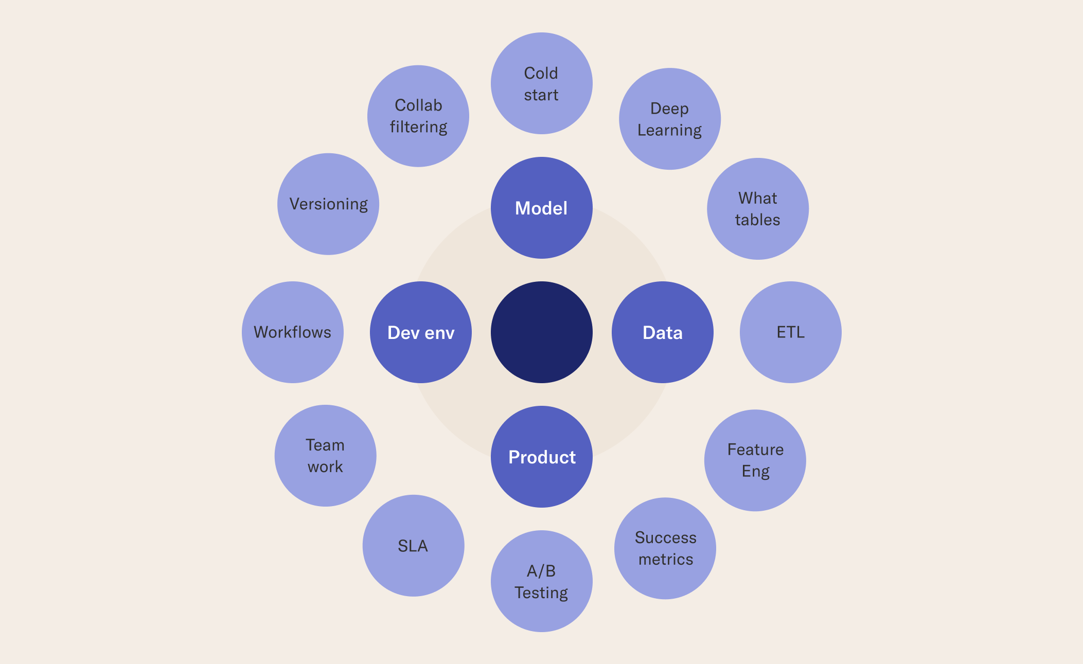
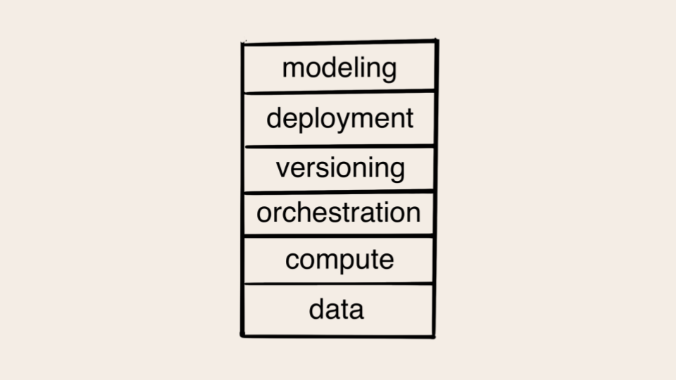

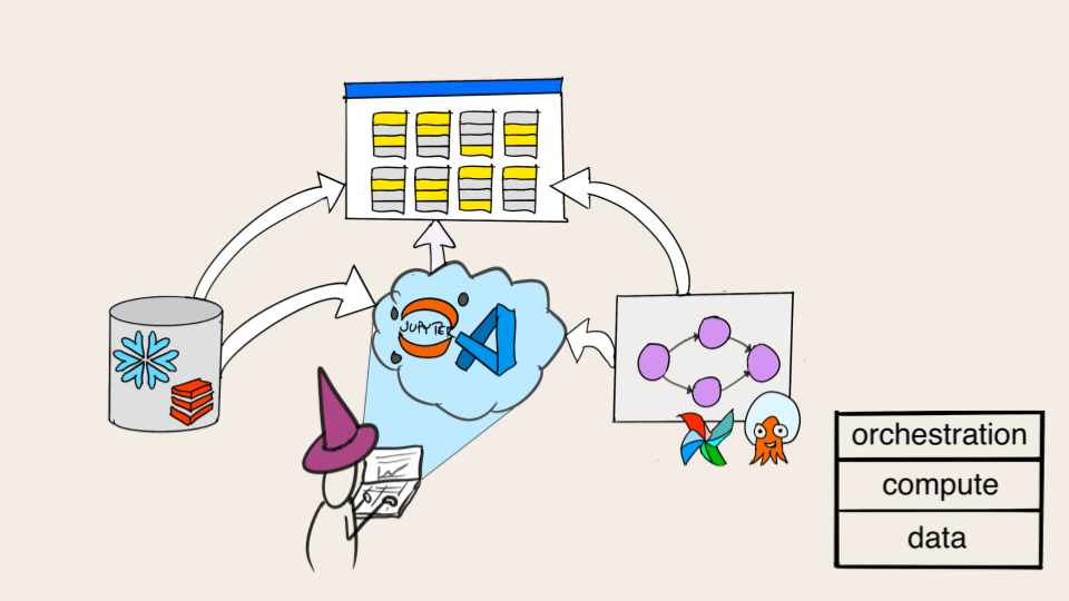
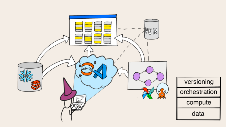
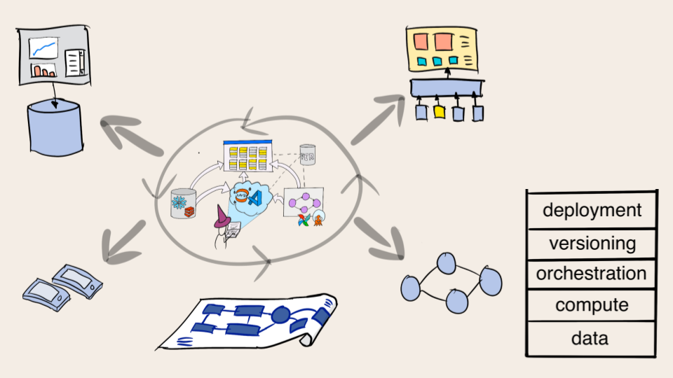
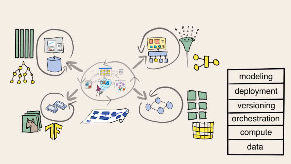
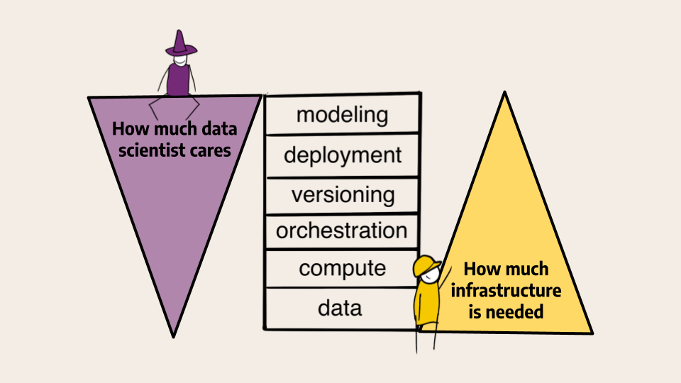
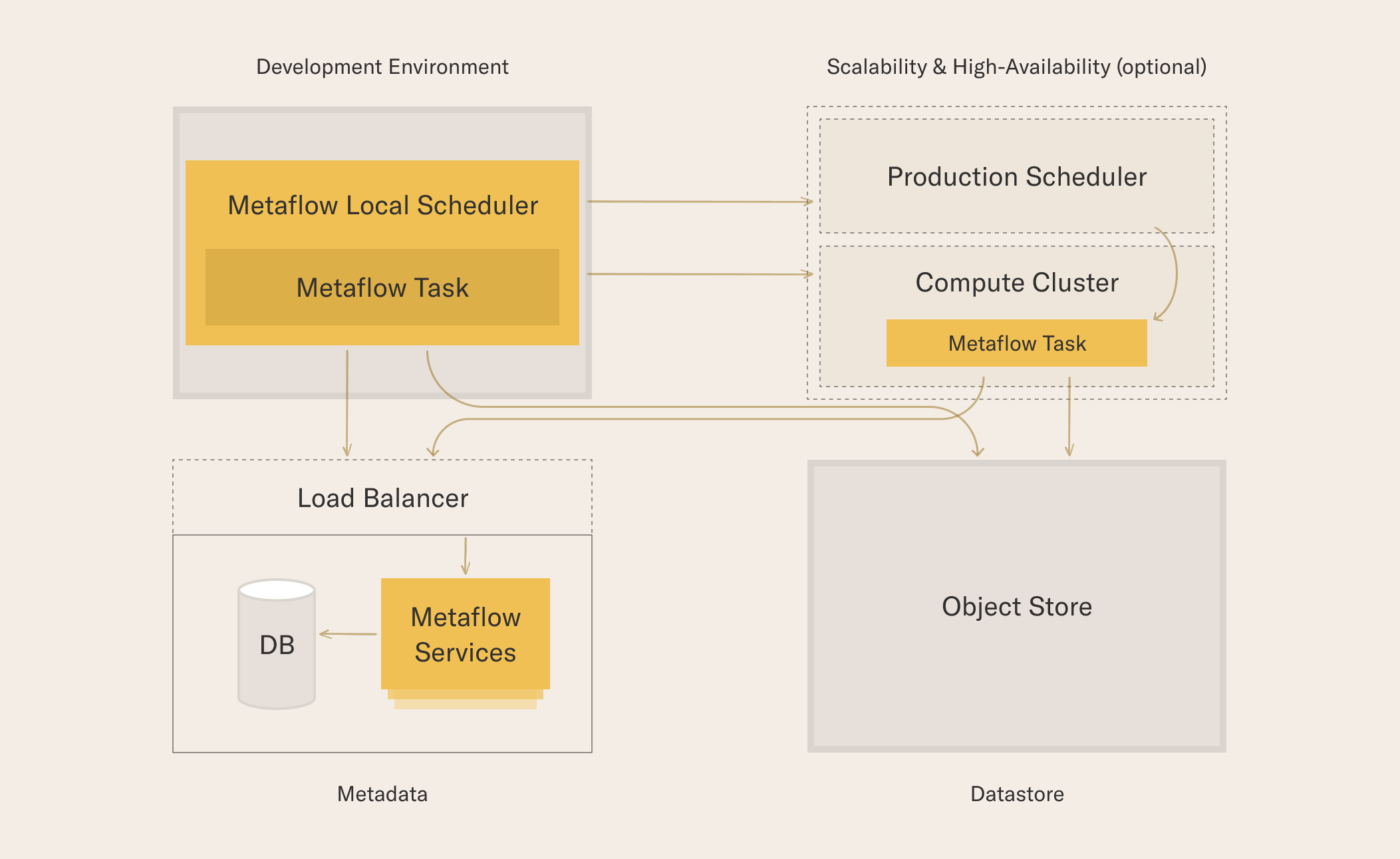
--- // File: engineering/deployment/aws-managed/terraform-deployment We support a [Terraform module](https://github.com/outerbounds/terraform-aws-metaflow) that automates the deployment of infrastructure to scale your Metaflow flows beyond your laptop. The module contains configuration for: - **Amazon S3** - A dedicated private bucket to serve as a centralized storage backend. - **AWS Batch** - A dedicated AWS Batch Compute Environment and Job Queue to extend Metaflow's compute capabilities to the cloud. - **Amazon CloudWatch** - Configuration to store and manage AWS Batch job execution logs. - **AWS Step Functions** - To allow scheduling Metaflow flows on AWS Step Functions. - **Amazon Event Bridge** - A dedicated role to allow time-based triggers for Metaflow flows configures on AWS Step Functions. - **Amazon DynamoDB** - A dedicated Amazon DynamoDB table for tracking certain step executions on AWS Step Functions. - **AWS Fargate and Amazon Relational Database Service** - A Metadata service running on AWS Fargate with a PostgresSQL DB on Amazon Relational Database Service to log flow execution metadata, as well as (optional) UI backend and front end app. - **Amazon API Gateway** - A dedicated TLS termination point and an optional point of basic API authentication via key to provide secure, encrypted access to the Metadata service. - **AWS Identity and Access Management** - Dedicated roles obeying "principle of least privilege" access to resources such as AWS Batch. - **AWS Lambda** _-_ An AWS Lambda function that automates database migrations for the Metadata service. This Terraform module consists of several submodules that can be used separately as well. You can see the details in the [README in the repository](https://github.com/outerbounds/terraform-aws-metaflow) ![modules diagram](/assets/terraform-batch.png) Resources used in Terraform Modules that deploy Metaflow with AWS Batch --- // File: engineering/deployment/azure-k8s/advanced Here are some advanced options for deploying Metaflow on Azure. ## Remote state backends for Terraform Terraform manages the state of Azure resources in tfstate files locally by default. If you plan to maintain the minimal stack for any significant period of time, it is highly recommended that these state files be stored in cloud storage (e.g. Azure Blob Storage) instead. Some reasons include: * More than one person needs to administer the stack (using Terraform). Everyone should work off a single copy of tfstate. * You wish to mitigate the risk of data loss on your local disk. For more details, see Terraform docs. ## Deploying Multiple Metaflow Stacks If you want to run more than one instance of this stack, you can use [Terraform workspaces](https://www.terraform.io/language/state/workspaces). ## Authenticated Public Endpoints for Metaflow Services The deployment approach taken by the terraform templates minimizes publicly accessible surface area. Only the AKS Kubernetes API is available publicly. This allows authorized users (through the secure Kubernetes API) to: * Inspect cluster's workloads * CRUD Kubernetes objects (e.g. submit job pods). However, this deployment style does not include publicly accessible endpoints for the [web services](/engineering/deployment/azure-k8s/details/#azure-services-list) running within the AKS cluster. For the purpose of this sample deployment template, users must use the Kubernetes API to set up port-forwarding in order to access these services from their workstations. For a more friendly user experience, publicly accessible endpoints can be authenticated and authorized using technologies like: * [OIDC](https://openid.net/connect/) (OpenID Connect) * [JWT](https://jwt.io/) tokens * Identity-as-a-service providers (e.g. [Auth0](https://auth0.com/)). Please [talk to us](http://slack.outerbounds.co) for more information about this topic. ## AKS Workload Identities In the Metaflow stack generated by these terraform templates, all Metaflow workloads running within AKS access Azure resources as a specific Service Principal identity. For finer grain control, it is possible to map separate identities to each workload and Metaflow task. The strategy currently recommended by Azure is [Azure AD Workload Identity](https://azure.github.io/azure-workload-identity/docs/). --- // File: engineering/deployment/azure-k8s/deployment This page shows how to deploy a complete [Metaflow stack](/engineering/service-architecture/) powered by Kubernetes on Microsoft Azure. For more information about the deployment, see [deployment details](/engineering/deployment/azure-k8s/details), [advanced options](/engineering/deployment/azure-k8s/advanced) and [FAQ](/engineering/deployment/azure-k8s/faq). ## 1. Preparation ### Terraform Tooling [Terraform](https://www.terraform.io/) is a popular infrastructure-as-code tool for managing cloud resources. We have published a set of Terraform templates [here](https://github.com/outerbounds/metaflow-tools/tree/master/azure/terraform) for setting up Metaflow on Microsoft Azure. Terraform needs to be installed on your system in order to use these templates. 1. Install Terraform by following [these instructions](https://learn.hashicorp.com/tutorials/terraform/install-cli). 2. Download [Metaflow on Azure terraform templates](https://github.com/outerbounds/metaflow-tools/tree/master/azure/terraform): ``` git clone git@github.com:outerbounds/metaflow-tools.git ``` ### Azure Command Line Interface This is the [official CLI tool ("az")](https://docs.microsoft.com/en-us/cli/azure/) published by Microsoft for working with Azure. It will be used by Terraform when applying our templates (e.g. for authentication with Azure). Please install it by following [these instructions](https://docs.microsoft.com/en-us/cli/azure/install-azure-cli). ### kubectl Command Line Interface [kubectl](https://kubernetes.io/docs/reference/kubectl/) is a standard CLI tool for working with [Kubernetes](https://kubernetes.io/) clusters. It will be used by Terraform when applying our templates (e.g. for deploying some services to your [Azure Kubernetes Service](https://azure.microsoft.com/en-us/services/kubernetes-service/) cluster). Please install it by following [these instructions](https://kubernetes.io/docs/tasks/tools/#kubectl). ## 2. Provision Azure Resources See here for the exact set of resources to be provisioned. Also, note the [permissions](/engineering/deployment/azure-k8s/details/#required-azure-permissions-for-running-flows) that are needed. ### Login to Azure You must be logged onto Azure as an account with [sufficient permissions](/engineering/deployment/azure-k8s/details/#required-azure-permissions-for-running-flows) to provision the required resources. Use the Azure CLI (`az`): ``` az login ``` ### Initialize your Terraform Workspace From your `metaflow-tools/azure/terraform` directory, run: ``` terraform init ``` ### Set org_prefix Create a TF vars file `FILE.tfvars` (`FILE` could be something else), with this content. org_prefix = "yourorg" # use something short and distinctive Some Azure resources must have globally unique names: - Azure storage account - Azure PostgreSQL Flexible Server `org_prefix` will be used to ensure this uniqueness. Uncomment [this line](https://github.com/outerbounds/metaflow-tools/blob/f7ff07d49563dc8217f7fe49150b2d50a14d999f/azure/terraform/variables.tf#L9), and set `org_prefix` to a value of your choice. Short and distinctive is best. #### Optional: Enable Argo Events To enable [event triggering](https://docs.metaflow.org/production/event-triggering) for Metaflow, add the following line in `FILE.tfvars`: ``` enable_argo=true ``` For more technical context, [see this page about event triggering](/engineering/operations/event-triggering/). #### Optional: Enable Airflow Optionally, you can include [Apache Airflow as the production orchestrator for Metaflow](https://docs.metaflow.org/production/scheduling-metaflow-flows/scheduling-with-airflow) in your deployment by including the following lines in `FILE.tfvars`: ``` deploy_airflow=true ``` Setting `deploy_airflow=true` will create a storage blob-container named `airflow-logs`, provide blob-container read and write permissions to the service principal and deploy Airflow in the AKS cluster with a `LocalExecutor`. The Airflow installation will store the logs in the `airflow-logs` blob container. ### Apply Terraform Template to Provision Azure Infrastructure From your local `metaflow-tools/azure/terraform directory`, run: ``` terraform apply -target="module.infra" -var-file="FILE.tfvars" ``` A plan of action will be printed to the terminal. You should review it before accepting. See [details](/engineering/deployment/azure-k8s/details/) for what to expect. ### Common Resource Provisioning Hiccups #### PostgreSQL Provisioning API Errors (on Azure Side) If you do not create Azure PostgreSQL Flexible Server instances often, Azure API may be flaky for you initially: ``` | Error: waiting for creation of the Postgresql Flexible Server "metaflow-database-server-xyz" (Resource Group "rg-db-metaflow-xyz"): | Code="InternalServerError" Message="An unexpected error occured while processing the request. Tracking ID: 'xyz'" | | with module.infra.azurerm_postgresql_flexible_server.metaflow_database_server, | on infra/database.tf line 20, in resource "azurerm_postgresql_flexible_server" "metaflow_database_server": | 20: resource "azurerm_postgresql_flexible_server" "metaflow_database_server" { ``` In our experience, waiting 20 mins and trying again resolves this issue. This appears to be a one-time phenomenon - future stack spin-ups do not encounter such `InternalServerError`s. #### Node Pool Provisioning We have hard-coded some default instance types to be used for Kubernetes nodes as well as worker pools (taskworkers). Depending on the real-time availability of such instances in your region or availability zone, you may [consider choosing alternate instance types](/engineering/deployment/azure-k8s/faq/#how-do-i-change-the-vm-instance-types-for-the-aks-control-plane-as-well-as-for-metaflow-task-runner-nodes). VM Availability issues might look something like this: ``` | Error: waiting for creation of Node Pool: (Agent Pool Name "taskworkers" / Managed Cluster Name "metaflow-kubernetes-xyz" / | Resource Group "rg-k8s-metaflow-xyz"): Code="ReconcileVMSSAgentPoolFailed" Message="Code=\"AllocationFailed\" Message=\"Allocation failed. | We do not have sufficient capacity for the requested VM size in this region. Read more about improving likelihood of allocation success | at http://aka.ms/allocation-guidance\"" ``` VM quotas may also cause provisioning to fail - we recommend working with your Azure admin to raise quotas, and/or pick other instance types: ``` | Error: creating Node Pool: (Agent Pool Name "taskworkers" / Managed Cluster Name "metaflow-kubernetes-default" / Resource Group "rg-k8s-metaflow-default"): | containerservice.AgentPoolsClient#CreateOrUpdate: Failure sending request: StatusCode=400 -- Original Error: Code="PreconditionFailed" | Message="Provisioning of resource(s) for Agent Pool taskworkers failed. Error: {\n \"code\": \"InvalidTemplateDeployment\",\n | \"message\": \"The template deployment '8b1a99f1-e35e-44be-a8ac-0f82009b7149' is not valid according to the validation procedure. | The tracking id is 'xyz'. See inner errors for details.\",\n \"details\": | [\n {\n \"code\": \"QuotaExceeded\",\n \"message\": \"Operation could not be completed as it results in exceeding approved standardDv5Family Cores quota. | Additional details - Deployment Model: Resource Manager, Location: westeurope, Current Limit: 0, Current Usage: 0, | Additional Required: 4, (Minimum) New Limit Required: 4. | Submit a request for Quota increase at https:// by specifying parameters listed in the ‘Details’ section for deployment to succeed. | Please read more about quota limits at https://docs.microsoft.com/en-us/azure/azure-supportability/per-vm-quota-requests\"\n }\n ]\n }" ``` ## 3. Deploy Metaflow Services to AKS Cluster ### Apply Terraform Template to Deploy Services From your local `metaflow-tools/azure/terraform` directory, run: ``` terraform apply -target="module.services" -var-file="FILE.tfvars" ``` ## 4. End User Setup Instructions When the command above completes, it will print a set of setup instructions for Metaflow end users (folks who will be writing and running flows). These instructions are meant to get end users started on running flows quickly. You can access the Terraform instruction output at any time by running (from `metaflow-tools/azure/terraform` directory): ``` terraform output -raw END_USER_SETUP_INSTRUCTIONS ``` ### Sample Output ``` Setup instructions for END USERS (e.g. someone running Flows vs the new stack): ------------------------------------------------------------------------------- There are three steps: 1. Ensuring Azure access 2. Configure Metaflow 3. Run port forwards 4. Install necessary Azure Python SDK libraries STEP 1: Ensure you have sufficient access to these Azure resources on your local workstation: - AKS cluster ("aks-ob-metaflow-minion") ("Azure Kubernetes Service Contributor" + "Azure Kubernetes Service Cluster User Role") - Azure Storage ("metaflow-storage-container" in the storage account "stobmetaflowminion") ("Storage Blob Data Contributor") You can use "az login" as a sufficiently capabable account. To see the credentials for the service principal (created by terraform) that is capable, run this: $ terraform output -raw SERVICE_PRINCIPAL_CREDENTIALS Use the credentials with "az login" $ az login --service-principal -u $AZURE_CLIENT_ID -p $AZURE_CLIENT_SECRET --tenant $AZURE_TENANT_ID Configure your local Kubernetes context to point to the the right Kubernetes cluster: $ az aks get-credentials --resource-group rg-metaflow-minion-westus --name aks-ob-metaflow-minion STEP 2: Configure Metaflow: $ metaflow configure azure $ metaflow configure kubernetes Use these values when prompted: METAFLOW_DATASTORE_SYSROOT_AZURE=metaflow-storage-container/tf-full-stack-sysroot METAFLOW_AZURE_STORAGE_BLOB_SERVICE_ENDPOINT=https://stobmetaflowminion.blob.core.windows.net/ METAFLOW_KUBERNETES_SECRETS=metaflow-azure-storage-credentials METAFLOW_SERVICE_URL=http://127.0.0.1:8080/ METAFLOW_SERVICE_INTERNAL_URL=http://metadata-service.default:8080/ [For Argo only] METAFLOW_KUBERNETES_NAMESPACE=argo Note: you can skip METAFLOW_SERVICE_AUTH_KEY (leave it blank) STEP 3: Setup port-forwards to services running on Kubernetes: option 1 - run kubectl's manually: $ kubectl port-forward deployment/metadata-service 8080:8080 $ kubectl port-forward deployment/metaflow-ui-backend-service 8083:8083 $ kubectl port-forward deployment/metaflow-ui-static-service 3000:3000 $ kubectl port-forward -n argo deployment/argo-server 2746:2746 option 2 - this script manages the same port-forwards for you (and prevents timeouts) $ python metaflow-tools/scripts/forward_metaflow_ports.py [--include-argo] STEP 4: Install Azure Python SDK $ pip install azure-storage-blob azure-identity ``` --- // File: engineering/deployment/azure-k8s/details Here are key technical details about the Metaflow deployment on Azure. ## Architecture Diagram ![](/assets/azure-architecture-diagram.png) ## Azure Resource List | Category | Resources | Purpose | | -------------- | ----------- | -------------------------------------- | | Resource Group | n/a | This will contain all resources directly created by the Terraform template.| | Access Control | Azure Active Directory Application | This represents Metaflow as an "app" that will access various Azure resources. More [info](https://docs.microsoft.com/en-us/azure/active-directory/develop/app-objects-and-service-principals). | | Access Control | Azure Active Directory Service Principal | This is an identity, linked to the AAD application above that will be used by the Metaflow application. More [info](https://docs.microsoft.com/en-us/azure/active-directory/develop/app-objects-and-service-principals). | | Access Control | Azure Active Directory Service Principal Password | This will be used by Metaflow to authenticate as the service principal above. | | Access Control | Role Assignments | Grant the service principal above sufficient access to Azure Blob Storage and AKS cluster. For specific details and conditions tied to these role assignments, please refer to the [source code](https://github.com/outerbounds/metaflow-tools/blob/f7ff07d49563dc8217f7fe49150b2d50a14d999f/azure/terraform/infra/credentials.tf#L21). | | Networking | Virtual network | Top-level private virtual network to house all Metaflow-related Azure resources. | | Networking | Subnets | There are two of these. One to house the PostgreSQL DB. One to house the AKS cluster. Both subnets live within the single virtual network above. | | Storage | Azure Storage Account | Dedicated storage account for use with Metaflow | | Storage | Azure Blob Storage container | Metaflow artifacts will be stored here. This resides within the storage account above. | | Kubernetes | AKS cluster | There are two purposes. One is that Metaflow services run on this cluster. The other is that compute tasks from running flows will be run as pods in this cluster. | | Kubernetes | AKS cluster node pool | A dedicated, autoscaling node pool for running services and tasks, distinct from AKS's Kubernetes control plane pods. | | Database | Azure PostgreSQL Flexible Server | This is a PostgreSQL DB instance for indexing Metaflow run metadata. | ## Required Azure Permissions for Deployment ### In Azure Active Directory Application Administrator role is required (Terraform [doc](https://registry.terraform.io/providers/hashicorp/azuread/latest/docs/resources/application)). We will be creating an Active Directory Application and a related Service Principal in the relevant Active Directory (AKA "tenant"). ![](/assets/azure-admin-roles.png) ### In Azure IAM Here is a custom role definition (JSON) containing all required permissions to manage the full lifecycle of a Metaflow-on-Azure stack using the Terraform templates. Note: "delete" type permissions are only needed for tearing down the stack ("terraform destroy"). ``` { "id": "", "properties": { "assignableScopes": [ "/subscriptions/" ], "description": "", "permissions": [ { "actions": [ "Microsoft.Resources/subscriptions/resourceGroups/read", "Microsoft.Resources/subscriptions/resourceGroups/write", "Microsoft.Network/privateDnsZones/read", "Microsoft.Network/privateDnsZones/write", "Microsoft.Network/privateDnsZones/SOA/read", "Microsoft.Storage/storageAccounts/read", "Microsoft.Network/virtualNetworks/read", "Microsoft.Network/virtualNetworks/write", "Microsoft.Storage/storageAccounts/write", "Microsoft.Network/virtualNetworks/subnets/read", "Microsoft.Network/virtualNetworks/subnets/write", "Microsoft.Storage/storageAccounts/listkeys/action", "Microsoft.Storage/storageAccounts/blobServices/read", "Microsoft.Storage/storageAccounts/blobServices/write", "Microsoft.Storage/storageAccounts/fileServices/read", "Microsoft.ContainerService/managedClusters/read", "Microsoft.ContainerService/managedClusters/write", "Microsoft.Network/virtualNetworks/subnets/join/action", "Microsoft.ContainerService/managedClusters/accessProfiles/listCredential/action", "Microsoft.Network/privateDnsZones/virtualNetworkLinks/read", "Microsoft.Authorization/roleAssignments/read", "Microsoft.ContainerService/managedClusters/agentPools/read", "Microsoft.ContainerService/managedClusters/agentPools/write", "Microsoft.Network/privateDnsZones/virtualNetworkLinks/write", "Microsoft.Authorization/roleAssignments/write", "Microsoft.Network/virtualNetworks/join/action", "Microsoft.DBforPostgreSQL/flexibleServers/read", "Microsoft.DBforPostgreSQL/flexibleServers/write", "Microsoft.DBforPostgreSQL/flexibleServers/databases/read", "Microsoft.DBforPostgreSQL/flexibleServers/databases/write", "Microsoft.DBforPostgreSQL/flexibleServers/configurations/read", "Microsoft.DBforPostgreSQL/flexibleServers/configurations/write", "Microsoft.ContainerService/managedClusters/listClusterUserCredential/action", "Microsoft.Authorization/roleAssignments/delete", "Microsoft.DBforPostgreSQL/flexibleServers/databases/delete", "Microsoft.ContainerService/managedClusters/agentPools/delete", "Microsoft.Storage/storageAccounts/delete", "Microsoft.ContainerService/managedClusters/delete", "Microsoft.DBforPostgreSQL/flexibleServers/delete", "Microsoft.Network/virtualNetworks/subnets/delete", "Microsoft.Network/privateDnsZones/virtualNetworkLinks/delete", "Microsoft.Network/virtualNetworks/delete", "Microsoft.Network/privateDnsZones/delete", "Microsoft.Resources/subscriptions/resourceGroups/delete" ], "dataActions": [], "notActions": [], "notDataActions": [] } ], "roleName": "Metaflow admin" } } ``` You can create a custom role as follows. From [Azure Portal](https://portal.azure.com), Go to Subscriptions => select the right subscription ⇒ Access Control (IAM), then choose the "Create custom role" panel on RHS. Paste in the role definition JSON. ![](/assets/azure-iam.png) ![](/assets/azure-custom-role.png) ## Required Azure Permissions for Running Flows ### Storage Access In the Azure portal, navigate to the relevant storage account/storage container. E.g. from this Terraform output: ``` METAFLOW_AZURE_STORAGE_BLOB_SERVICE_ENDPOINT=https://stobmetaflowminion.blob.core.windows.net/ METAFLOW_DATASTORE_SYSROOT_AZURE=metaflow-storage-container/tf-full-stack-sysroot ``` `stobmetaflowminion` is the storage account, `metaflow-storage-container` is the storage container. From the container page, go to "Access Control (IAM)" to assign the role *Storage Blob Data Contributor*). Note this role assignment can take several minutes to propagate in our experience. ### AKS Cluster Access In Azure portal, navigate to the relevant AKS cluster. E.g. from this Terraform output: ``` az aks get-credentials --resource-group rg-metaflow-minion-westus --name aks-ob-metaflow-minion ``` `aks-ob-metaflow-minion` is the AKS cluster name. Navigate to the management for this cluster, and go to "Access Control (IAM)" to assign the roles: * *Azure Kubernetes Service Contributor Role* * *Azure Kubernetes Service Cluster User Role* ## Azure Services List We deploy these services in the AKS cluster: ### Metaflow * Metadata service - this supports read/write of metadata. Supports features such as: * When a flow is running, it POST's metadata here. * The Metaflow Client library calls this service to read metadata. * The UI static service serves the web UI frontend bundle. * The UI backend supports UI's data needs. ### Argo Workflows The [quickstart](https://argoproj.github.io/argo-workflows/quick-start/) k8s manifest published by Argo Workflows spins up the following services: ``` kubectl get services -n argo NAME TYPE CLUSTER-IP EXTERNAL-IP PORT(S) AGE argo-server ClusterIP 10.0.26.126 2746/TCP 32m httpbin ClusterIP 10.0.66.229 9100/TCP 32m minio ClusterIP 10.0.173.242 9000/TCP,9001/TCP 32m postgres ClusterIP 10.0.51.199 5432/TCP 32m workflow-controller-metrics ClusterIP 10.0.139.237 9090/TCP 32m ``` --- // File: engineering/deployment/azure-k8s/faq ### What's with all the port forwards? See [here](/engineering/deployment/azure-k8s/advanced/#authenticated-public-endpoints-for-metaflow-services). We publish a short utility script to open up the port forwards and keep them open by preventing inactivity timeouts [here](https://github.com/outerbounds/metaflow-tools/blob/master/scripts/forward_metaflow_ports.py). ### I want to use an existing storage account/container, an existing AKS, or DB. What to do? The terraform templates provide an all-in experience, spinning up all fresh resources. The templates need to be adapted to accommodate existing resources. E.g. to bring your own storage account and storage container, here are some possible approaches: *Full manual reference replacement* * Look for all references to the terraform resources: * `metaflow_storage_account` * `metaflow_storage_container` * Replace references with known attributes of the account and container you are bringing. E.g. storage_account_name, or container_name, etc. * Remove terraform resources for `metaflow_storage_account` and `metaflow_storage_container` from templates. *Terraform "data source" approach* * Replace the resources `metaflow_storage_account` and `metaflow_storage_container` with "[data sources](https://www.terraform.io/language/data-sources)". I.e. [storage_container](https://registry.terraform.io/providers/hashicorp/azurerm/latest/docs/data-sources/storage_container), [storage_account](https://registry.terraform.io/providers/hashicorp/azurerm/latest/docs/data-sources/storage_account). * Update references to these resources, so that the callers refer to the "data source" object instead. I.e. `data.storage_account.`. ### How do I use GPU nodes in my AKS cluster? Our quickstart terraform templates will not support that out of the box. They may be extended in the future. The approach would likely implement [this](https://docs.microsoft.com/en-us/azure/aks/gpu-cluster) in an automated manner within the templates. ### How do I change the VM instance types for the AKS control plane as well as for Metaflow task runner nodes? Change these lines ([control plane](https://github.com/outerbounds/metaflow-tools/blob/3048eb1e4ac1b0d32c4ad9e73249385b813ef772/azure/terraform/infra/kubernetes.tf#L9), [tasks](https://github.com/outerbounds/metaflow-tools/blob/3048eb1e4ac1b0d32c4ad9e73249385b813ef772/azure/terraform/infra/kubernetes.tf#L40)) and reapply the Terraform template ("`terraform apply -target=module.infra`") ### I want finer grain auth on running flows. What to do? See [here](/engineering/deployment/azure-k8s/advanced/#aks-workload-identities). ### Why is my Metaflow flow stuck on k8s pending state forever? When Metaflow submits tasks to Kubernetes for execution, there are two scenarios: * There are sufficient spare resources to immediately run the task. * There are NOT sufficient spare resources right now. AKS autoscaler provisions additional compute nodes to satisfy the requirements of the new task. Once provisioning is complete, the task is run. The AKS autoscaler is configured with a specific instance type (defaults to Standard_D8_v5) to provision if needed. If a task's resource requirements exceed the VM size, upscaling can never satisfy the new task and the task will be stuck in pending forever. When this is suspected, double-check your resource requirements vs the VM instance type used in the *taskworker* node pool. ### Can I do the deployment quickstart on Windows? Yes, all the CLI tools involved work on Windows natively. ## Need Help? The quickest way to get help is our public Slack channel [#ask-metaflow](http://slack.outerbounds.co). We look forward to your questions and feedback. --- // File: engineering/deployment/gcp-k8s/advanced Here are some advanced options for deploying Metaflow on Google Cloud. ## Remote State Backends for Terraform Terraform manages the state of GCP resources in [tfstate](https://www.terraform.io/language/state) files locally by default. If you plan to maintain the minimal stack for any significant period of time, it is highly recommended that these state files be stored in cloud storage (e.g. Google Cloud Storage) instead. Some reasons include * More than one person needs to administer the stack (using terraform). Everyone should work off a single copy of tfstate. * You wish to mitigate the risk of data loss on your local disk. For more details, see [Terraform docs](https://www.terraform.io/language/settings/backends/configuration). ## Deploying Multiple Metaflow Stacks If you want to run more than one instance of this stack, you can use [Terraform workspaces](https://www.terraform.io/language/state/workspaces). ## Authenticated Public Endpoints for Metaflow Services The deployment approach taken by the terraform templates minimizes publicly accessible surface area. Only the GKE Kubernetes API is available publicly. This allows authorized users (through the secure Kubernetes API) to * Inspect cluster's workloads * CRUD Kubernetes objects (e.g. submit job pods) However, this deployment style does not include publicly accessible endpoints for the [web services](https://docs.google.com/document/d/19kQc0fpC7PWUiJoyb-vS41wTG_T1_p61gagGmnbM45I/edit#heading=h.lziyyitnsxax) running within the GKE cluster. For the purpose of this sample deployment template, users must use the Kubernetes API to set up port-forwarding in order to access these services from their workstations. For a more friendly user experience, publicly accessible endpoints can be authenticated and authorized using technologies like: * [OIDC](https://openid.net/connect/) (OpenID Connect) * [JWT](https://jwt.io/) tokens * Identity-as-a-service providers (e.g. [Auth0](https://auth0.com/)). Please [talk to us](http://slack.outerbounds.co) for more information about this topic. ## GKE Workload Identities In the Metaflow stack generated by these terraform templates, all Metaflow workloads running within GKE access GCP resources as a specific service account identity. We use [GKE Workload Identity](https://cloud.google.com/kubernetes-engine/docs/how-to/workload-identity) (in short), which does the following: * Metaflow tasks pods run as a certain Kubernetes Service Account (KSA) * KSA is annotated with a link to the Google Service Account (GSA) * The pod running as KSA assumes the identity of GSA when access GCP resources For finer grain control, it is possible to map separate identities to each workload and Metaflow task. It is possible to extend this further. E.g. user X's Metaflow runs may assume a certain KSA_1 (mapping to GSA_1), whilst user Y's Metaflow runs may assume a certain KSA_2 (mapping to GSA_2). --- // File: engineering/deployment/gcp-k8s/deplyoment This page shows how to deploy a complete Metaflow stack powered by Kubernetes on Google Cloud. For more information about the deployment, see [deployment details](/engineering/deployment/gcp-k8s/details), [advanced options](/engineering/deployment/gcp-k8s/advanced) and [FAQ](/engineering/deployment/gcp-k8s/faq). ## 1. Preparation ### Terraform Tooling [Terraform](https://www.terraform.io/) is a popular infrastructure-as-code tool for managing cloud resources. We have published a set of terraform templates [here](https://github.com/outerbounds/metaflow-tools/tree/master/azure/terraform) for setting up Metaflow on GCP. Terraform needs to be installed on your system in order to use these templates. 1. Install terraform by following [these instructions](https://learn.hashicorp.com/tutorials/terraform/install-cli). 2. Download [Metaflow on GCP terraform templates](https://github.com/outerbounds/metaflow-tools/tree/master/gcp/terraform): `git clone git@github.com:outerbounds/metaflow-tools.git` ### GCloud Command Line Interface This is the [official CLI tool ("gcloud")](https://cloud.google.com/sdk/gcloud) published by Google for working with GCP. It will be used by Terraform when applying our templates (e.g. for authentication vs GCP). Please install it by following [these instructions](https://cloud.google.com/sdk/docs/install-sdk). ### kubectl Command Line Interface [kubectl](https://kubernetes.io/docs/reference/kubectl/) is a standard CLI tool for working with [Kubernetes](https://kubernetes.io/) clusters. It will be used by Terraform when applying our templates (e.g. for deploying some services to your [Google Kubernetes Engine (GKE)](https://cloud.google.com/kubernetes-engine) cluster). Please install it by following [these instructions](https://kubernetes.io/docs/tasks/tools/#kubectl). ## 2. Provision GCP Resources See [here](/engineering/deployment/gcp-k8s/details/#gcp-resource-list) for the exact set of resources to be provisioned. Also, note the [permissions](/engineering/deployment/gcp-k8s/details/#required-gcp-permissions-for-deployment) that are needed. ### Enable Google Cloud APIs You need to manually enable APIs used by the Metaflow stack on the Google Cloud console. Make sure that the following APIs are enabled: - Cloud Resource Manager - Compute Engine API - Service Networking - Cloud SQL Admin API - Kubernetes Engine API If you have used the account/project for other deployments in the past, it is possible that these APIs are already enabled. Also note that enabling these APIs automatically enables a bunch of other required APIs. ### Login to GCP You must be logged onto GCP as an account with [sufficient permissions](/engineering/deployment/gcp-k8s/details/#required-gcp-permissions-for-deployment) to provision the required resources. Use the GCloud CLI (`gcloud`) ``` gcloud auth application-default login ``` ### Initialize your Terraform Workspace From your `metaflow-tools/gcp/terraform directory`, run: ``` terraform init ``` ### Set Terraform Variables Create a `FILE.tfvars` file with the following content (updating relevant values): ``` org_prefix = "" project = "" ``` For `org_prefix`, choose a short and memorable alphanumeric string. It will be used for naming the Google Cloud Storage bucket, whose name must be globally unique across GCP. For `GCP_PROJECT_ID`, set the GCP project ID you wish to use. You may rename `FILE.tfvars` to a more friendly name appropriate for your project. E.g. `metaflow.poc.tfvars`. The variable assignments defined in this file will be passed to `terraform` CLI. #### Optional: Enable Argo Events To enable [event triggering](https://docs.metaflow.org/production/event-triggering) for Metaflow, add the following line in `FILE.tfvars`: ``` enable_argo=true ``` For more technical context, [see this page about event triggering](/engineering/operations/event-triggering/). #### Optional: Enable Airflow Optionally, you can include [Apache Airflow as the production orchestrator for Metaflow](https://docs.metaflow.org/production/scheduling-metaflow-flows/scheduling-with-airflow) in your deployment by including the following lines in `FILE.tfvars`: ``` deploy_airflow=true ``` Setting `deploy_airflow=true` will deploy Airflow in the GKE cluster with a `LocalExecutor`. ### Apply Terraform Template to Provision GCP Infrastructure From your local `metaflow-tools/gcp/terraform` directory, run: ``` terraform apply -target="module.infra" -var-file=FILE.tfvars ``` A plan of action will be printed to the terminal. You should review it before accepting. See [details](/engineering/deployment/gcp-k8s/details/) for what to expect. ### Common Resource Provisioning Hiccups #### Cloud SQL instance name conflicts Cloud SQL instance (the "PostgreSQL DB") names must be unique within your GCP project - including instances that have been deleted within the last 7 days. It means that if you should want to reprovision the entire set of GCP resources within that time window, a fresh name must be chosen. In this scenario, please update the DB generation variable [here](https://github.com/outerbounds/metaflow-tools/blob/26c338860b9725cf5c8689036e4581781e12fbda/gcp/terraform/variables.tf#L9). ## 3. Deploy Metaflow Services to GKE cluster ### Apply Terraform Template to Deploy Services From your local `metaflow-tools/gcp/terraform` directory, run: ``` terraform apply -target="module.services" -var-file=FILE.tfvars ``` ## 4. End User Setup Instructions When the command above completes, it will print a set of setup instructions for Metaflow end users (folks who will be writing and running flows). These instructions are meant to get end users started on running flows quickly. You can access the terraform instruction output at any time by running (from `metaflow-tools/gcp/terraform directory`): ``` terraform output -raw END_USER_SETUP_INSTRUCTIONS ``` If the output is not available, run ``` terraform apply -var-file=FILE.tfvars ``` and try the `output` command again. ### Sample Output ``` Setup instructions for END USERS (e.g. someone running Flows vs the new stack): ------------------------------------------------------------------------------- There are three steps: 1. Ensuring GCP access 2. Configure Metaflow 3. Run port forwards 4. Install necessary GCP Python SDK libraries STEP 1: Ensure you have sufficient access to these GCP resources on your local workstation: - Google Kubernetes Engine ("Kubernetes Engine Developer role") - Google Cloud Storage ("Storage Object Admin" on bucket ob-metaflow-storage-bucket-ci) Option 1: Login with gcloud CLI Login as a sufficiently capabable user: $ gcloud auth application-default login. Option 2: Use service account key Ask for the pregenerated service account key (./metaflow_gsa_key_ci.json) from the administrator (the person who stood up the Metaflow stack). Save the key file locally to your home directory. It should be made to be accessible only by you (chmod 700 ) Configure your local Kubernetes context to point to the the right Kubernetes cluster: $ gcloud container clusters get-credentials metaflow-kubernetes-ci --region=us-west2 STEP 2: Configure Metaflow: Option 1: Create JSON config directly (recommended) Create the file "~/.metaflowconfig/config.json" with this content. If this file already exists, keep a backup of it and move it aside first. { "METAFLOW_DATASTORE_SYSROOT_GS": "gs://ob-metaflow-storage-bucket-ci/tf-full-stack-sysroot", "METAFLOW_DEFAULT_DATASTORE": "gs", "METAFLOW_DEFAULT_METADATA": "service", "METAFLOW_KUBERNETES_NAMESPACE": "default", "METAFLOW_KUBERNETES_SERVICE_ACCOUNT": "metaflow-service-account", "METAFLOW_SERVICE_INTERNAL_URL": "http://metadata-service.default:8080/", "METAFLOW_SERVICE_URL": "http://127.0.0.1:8080/" } Option 2: Interactive configuration Run the following, one after another. $ metaflow configure gs $ metaflow configure kubernetes Use these values when prompted: METAFLOW_DATASTORE_SYSROOT_GS=gs://ob-metaflow-storage-bucket-ci/tf-full-stack-sysroot METAFLOW_SERVICE_URL=http://127.0.0.1:8080/ METAFLOW_SERVICE_INTERNAL_URL=http://metadata-service.default:8080/ [For Argo only] METAFLOW_KUBERNETES_NAMESPACE=argo [For Argo only] METAFLOW_KUBERNETES_SERVICE_ACCOUNT=argo Note: you can skip these: METAFLOW_SERVICE_AUTH_KEY METAFLOW_KUBERNETES_CONTAINER_REGISTRY METAFLOW_KUBERNETES_CONTAINER_IMAGE STEP 3: Setup port-forwards to services running on Kubernetes: option 1 - run kubectl's manually: $ kubectl port-forward deployment/metadata-service 8080:8080 $ kubectl port-forward deployment/metaflow-ui-backend-service 8083:8083 $ kubectl port-forward deployment/metadata-service 3000:3000 $ kubectl port-forward -n argo deployment/argo-server 2746:2746 option 2 - this script manages the same port-forwards for you (and prevents timeouts) $ python metaflow-tools/scripts/forward_metaflow_ports.py [--include-argo] STEP 4: Install GCP Python SDK $ pip install google-cloud-storage google-auth ``` --- // File: engineering/deployment/gcp-k8s/details Here are key technical details about the Metaflow deployment on Google Cloud. ## Architecture Diagram ![](/assets/gke-architecture-diagram.png) ## GCP Resource List | Category | Resources | Purpose | | -------------- | ----------- | -------------------------------------- | | Access Control | Service account | This is an identity that has all required permissions to run Metaflow workloads, either locally vs Google Cloud Storage, or all the way running in the GKE cluster. More [info](https://cloud.google.com/kubernetes-engine/docs/how-to/workload-identity). | | Access Control | Service account key | This will be used by Metaflow to authenticate as the service account above. Note: This is needed for local runs as well as for Metaflow logic prior to workload tasks to GKE. For all GCP accesses from within a GKE pod, this credential is not required.| | Access Control | Role Assignments | Grants the service account above sufficient access to: Google Cloud Storage, GKE, and Cloud SQL (PostgreSQL). For specific details and conditions tied to these role assignments, please refer to the [source code](https://github.com/outerbounds/metaflow-tools/blob/master/gcp/terraform/infra/google_service_account.tf). | | Networking | Virtual network | Top-level private virtual network to house all Metaflow-related GCP resources. | | Networking | Subnet | To house the PostgreSQL DB | | Storage | Google Cloud Storage bucket | Metaflow artifacts will be stored here. This resides within the storage account above. | | Kubernetes | GKE cluster |This has built-in compute node autoscaling. There are two purposes. First, Metaflow services run on this cluster. Second, compute tasks from running flows will be run as pods in this cluster. | | Database | Cloud SQL instance | This is a PostgreSQL DB instance for indexing Metaflow run metadata. | ## Required GCP Permissions for Deployment The permissions required can be described by the following custom role (`gcloud iam roles describe` output): ``` description: includedPermissions: - cloudsql.backupRuns.create - cloudsql.backupRuns.delete - cloudsql.backupRuns.get - cloudsql.backupRuns.list - cloudsql.databases.create - cloudsql.databases.delete - cloudsql.databases.get - cloudsql.databases.list - cloudsql.databases.update - cloudsql.instances.addServerCa - cloudsql.instances.clone - cloudsql.instances.connect - cloudsql.instances.create - cloudsql.instances.createTagBinding - cloudsql.instances.delete - cloudsql.instances.deleteTagBinding - cloudsql.instances.demoteMaster - cloudsql.instances.export - cloudsql.instances.failover - cloudsql.instances.get - cloudsql.instances.import - cloudsql.instances.list - cloudsql.instances.listEffectiveTags - cloudsql.instances.listServerCas - cloudsql.instances.listTagBindings - cloudsql.instances.login - cloudsql.instances.promoteReplica - cloudsql.instances.resetSslConfig - cloudsql.instances.restart - cloudsql.instances.restoreBackup - cloudsql.instances.rotateServerCa - cloudsql.instances.startReplica - cloudsql.instances.stopReplica - cloudsql.instances.truncateLog - cloudsql.instances.update - cloudsql.sslCerts.create - cloudsql.sslCerts.delete - cloudsql.sslCerts.get - cloudsql.sslCerts.list - cloudsql.users.create - cloudsql.users.delete - cloudsql.users.get - cloudsql.users.list - cloudsql.users.update - compute.globalAddresses.createInternal - compute.globalAddresses.deleteInternal - compute.globalAddresses.get - compute.instanceGroupManagers.get - compute.networks.create - compute.networks.delete - compute.networks.get - compute.networks.removePeering - compute.networks.updatePolicy - compute.networks.use - compute.subnetworks.create - compute.subnetworks.delete - compute.subnetworks.get - container.clusterRoleBindings.create - container.clusterRoleBindings.delete - container.clusterRoleBindings.get - container.clusterRoleBindings.list - container.clusterRoleBindings.update - container.clusterRoles.bind - container.clusterRoles.create - container.clusterRoles.delete - container.clusterRoles.escalate - container.clusterRoles.get - container.clusterRoles.list - container.clusterRoles.update - container.clusters.create - container.clusters.delete - container.clusters.get - container.configMaps.create - container.configMaps.delete - container.configMaps.get - container.configMaps.list - container.configMaps.update - container.customResourceDefinitions.create - container.customResourceDefinitions.delete - container.customResourceDefinitions.get - container.customResourceDefinitions.getStatus - container.customResourceDefinitions.list - container.customResourceDefinitions.update - container.customResourceDefinitions.updateStatus - container.deployments.create - container.deployments.delete - container.deployments.get - container.deployments.getScale - container.deployments.getStatus - container.deployments.list - container.deployments.rollback - container.deployments.update - container.deployments.updateScale - container.deployments.updateStatus - container.namespaces.create - container.namespaces.delete - container.namespaces.finalize - container.namespaces.get - container.namespaces.getStatus - container.namespaces.list - container.namespaces.update - container.namespaces.updateStatus - container.operations.get - container.priorityClasses.create - container.priorityClasses.delete - container.priorityClasses.get - container.priorityClasses.list - container.priorityClasses.update - container.roleBindings.create - container.roleBindings.delete - container.roleBindings.get - container.roleBindings.list - container.roleBindings.update - container.roles.bind - container.roles.create - container.roles.delete - container.roles.escalate - container.roles.get - container.roles.list - container.roles.update - container.secrets.create - container.secrets.delete - container.secrets.get - container.secrets.list - container.secrets.update - container.serviceAccounts.create - container.serviceAccounts.createToken - container.serviceAccounts.delete - container.serviceAccounts.get - container.serviceAccounts.list - container.serviceAccounts.update - container.services.create - container.services.delete - container.services.get - container.services.getStatus - container.services.list - container.services.proxy - container.services.update - container.services.updateStatus - edgecontainer.clusters.create - iam.serviceAccountKeys.create - iam.serviceAccountKeys.get - iam.serviceAccounts.actAs - iam.serviceAccounts.create - iam.serviceAccounts.delete - iam.serviceAccounts.get - iam.serviceAccounts.getIamPolicy - iam.serviceAccounts.list - iam.serviceAccounts.setIamPolicy - resourcemanager.projects.get - resourcemanager.projects.setIamPolicy - servicenetworking.services.addPeering - servicenetworking.services.get - storage.buckets.create - storage.buckets.delete - storage.buckets.get - storage.objects.delete - storage.objects.list name: projects//roles/metaflow_admin stage: GA title: Metaflow admin ``` ## Required GCP Permissions for Running Flows ### Kubernetes Engine Developer Role Note: as of Q3, 2022, there is no direct way to scope this to a specific GKE cluster. ### Storage Object Admin Role This should be granted under this IAM condition: ``` resource.name.startsWith("projects/_/buckets/") ``` The bucket name can be found from the end user output from Terraform run. For example, ``` … "METAFLOW_DATASTORE_SYSROOT_GS": "gs://ob-metaflow-storage-bucket-ci/tf-full-stack-sysroot", … ``` ## GKE services list We deploy these services in the GKE cluster: ### Metaflow * Metadata service - this supports read/write of metadata. Supports features such as: * When flow is running, it POST's metadata here. * Metaflow Client library calls this service to read metadata. * The UI static service serves the web UI frontend bundle. * The UI backend supports UI's data needs. ### Argo Workflows The [quickstart](https://argoproj.github.io/argo-workflows/quick-start/) Kubernetes manifest published by Argo Workflows spins up the following services: ``` kubectl get services -n argo NAME TYPE CLUSTER-IP EXTERNAL-IP PORT(S) AGE argo-server ClusterIP 10.0.26.126 2746/TCP 32m httpbin ClusterIP 10.0.66.229 9100/TCP 32m minio ClusterIP 10.0.173.242 9000/TCP,9001/TCP 32m postgres ClusterIP 10.0.51.199 5432/TCP 32m workflow-controller-metrics ClusterIP 10.0.139.237 9090/TCP 32m ``` --- // File: engineering/deployment/gcp-k8s/faq ### What's with all the port forwards? See [here](/engineering/deployment/gcp-k8s/advanced/#authenticated-public-endpoints-for-metaflow-services). We publish a short utility script to open up the port forwards and keep them open by preventing inactivity timeouts [here](https://github.com/outerbounds/metaflow-tools/blob/master/scripts/forward_metaflow_ports.py). ### I want to use an existing storage account/container, an existing GKE, or DB. What to do? The terraform templates provide an all-in experience, spinning up all fresh resources. The templates need to be adapted to accommodate existing resources. E.g. to bring your own storage account and storage container, here are some possible approaches: *Full manual reference replacement:* * Look for all references to `metaflow_storage_bucket` * Replace references with known attributes of the account and container you are bringing. E.g. storage_account_name, or container_name, etc. * Remove terraform resources for `metaflow_storage_bucket` from templates. * Terraform "data source" approach:* * Replace the resources `metaflow_storage_bucket` with "data sources". i.e. [storage_bucket](https://registry.terraform.io/providers/hashicorp/google/latest/docs/data-sources/storage_bucket) * Update references to these resources, so that the callers refer to the "data source" object instead. I.e. `data.storage_bucket.` ### How do I use GPU nodes in my GKE cluster? Our quickstart terraform templates will not support that out of box. They may be extended in the future. The approach would likely implement [this](https://cloud.google.com/kubernetes-engine/docs/how-to/gpus) in an automated manner within the templates. ### How do I change the VM instance types for Metaflow task runner nodes? The quickstart terraform templates provided use GKE's [node auto-provisioning](https://cloud.google.com/kubernetes-engine/docs/how-to/node-auto-provisioning), out of the box. Node auto provisioning should be aware of the resource requirements of incoming pods, which means it will spin up appropriately sized instances as needed. ### I want finer grain auth on running flows. What to do? See [here](https://docs.google.com/document/d/19kQc0fpC7PWUiJoyb-vS41wTG_T1_p61gagGmnbM45I/edit#heading=h.4serr1lx4hxo). ### Why is my Metaflow flow stuck on k8s pending state forever? When Metaflow submits tasks to Kubernetes for execution, there are two scenarios: * There are sufficient spare resources to immediately run the task. * There are NOT sufficient spare resources right now. GKE autoscaler provisions additional compute nodes to satisfy the requirements of the new task. Once provisioning is complete, the task is run. If GKE autoscaler (running [node auto-provisioning](https://cloud.google.com/kubernetes-engine/docs/how-to/node-auto-provisioning)) can never satisfy the new task and the task will be stuck in pending forever. E.g. if the aggregate hard CPU or memory limit has been reached on the GKE cluster. To resolve the aggregate limit issue, up the limit in the [templates](https://github.com/outerbounds/metaflow-tools/blob/26c338860b9725cf5c8689036e4581781e12fbda/gcp/terraform/infra/kubernetes.tf#L29). ### Need Help? The quickest way to get help is our public Slack channel [#ask-metaflow](http://slack.outerbounds.co). We look forward to your questions and feedback. --- // File: engineering/eng-index These resources help you set up and operate [the full stack of ML/data science infrastructure](/docs/infra-stack/) for [Metaflow](https://docs.metaflow.org). If you are new to Metaflow or the topic in general, take a look at [Metaflow Resources for Data Science](/data-science-welcome/) first. To get started with setting up the Metaflow stack, choose a deployment option below. For background, see [an overview of supported Metaflow stacks](https://docs.metaflow.org/getting-started/infrastructure) and [Motivation](/engineering/motivation/).
--- Once you have deployed the stack, take a look at [Operating Metaflow](/engineering/operations/introduction/) for operational guidance. If you need help with anything, join [the Metaflow support Slack](http://slack.outerbounds.co) for quick and friendly advice! ![](/assets/engineering-welcome-01.png) --- // File: engineering/eng-overview Since the early days of Metaflow at Netflix, Metaflow has been designed to be the common layer that [binds together infrastructure components, people, and projects](https://docs.metaflow.org/introduction/why-metaflow). This documentation is targeted at systems administrators who want to deploy and operate such a stack for their organization. One of the core tenets of Metaflow is fanatic focus on usability and ergonomics. Besides being delightful to use, we want Metaflow to be delightfully simple to operate at scale. From experience, we know that much of the pain related to operating modern machine learning infrastructure is caused by the complexity of large-scale distributed systems. While some of this pain is inherent in nature - complex systems are complex - there's plenty of accidental complexity in many systems which we can avoid. Metaflow comes with a number of design choices that make it easy to operate, regardless of whether you have a handful or hundreds of data scientists using Metaflow: * Metaflow is designed from the ground up to leverage elastic storage and compute services available in the cloud without introducing bottlenecks. Metaflow scales as well as your cloud provider. * All user-facing functionality is provided as a library that provides strong guarantees for backwards-compatibility which implies no migration overhead between versions. Users can safely upgrade the library without having to fear that their projects break unintentionally. * Only one simple backend service is required which tracks relatively lightweight metadata so it can scale to hundreds of users and millions of executions with minimal operational overhead. It is easy to deploy on various container platforms. * The Metaflow deployment can be easily configured to comply with security and data governance requirements of your organization. Metaflow relies on proven cloud-native governance concepts instead of trying to reinvent the wheel. * Metaflow handles both frictionless prototyping as well as production-grade deployments to highly-available schedulers. Metaflow’s approach makes it possible to define organization-wide policies and best practices while leaving plenty of freedom for data scientists to do their job well. ## Learn more See these resources to learn more about the internals of Metaflow: - [Overview of Metaflow Stacks](https://docs.metaflow.org/getting-started/infrastructure) - [Service Architecture](/engineering/service-architecture/) - [Internals of Metaflow](https://docs.metaflow.org/internals/technical-overview) --- // File: engineering/getting-in-touch We know that deploying and operating infrastructure can be tricky. We are here to help. There are several ways to get in touch with us: * Open an issue at: [github.com/Netflix/metaflow](http://github.com/Netflix/metaflow) * Email us at: [help@metaflow.org](mailto:help@metaflow.org) * Chat with us on: [http://chat.metaflow.org](http://slack.outerbounds.co/) --- // File: engineering/operations/airflow You can deploy workflows developed with Metaflow on Apache Airflow, a popular open-source workflow orchestrator. For background why the integration exists in the first place, [see the Metaflow-Airflow announcement post](https://outerbounds.com/blog/better-airflow-with-metaflow/). For user-facing documentation, see [Scheduling Metaflow Flows with Apache Airflow](https://docs.metaflow.org/production/scheduling-metaflow-flows/scheduling-with-airflow). This section dives deeper in technical details of the integration, which may be useful for engineers who operate Airflow and Metaflow. ## How to deploy Airflow for Metaflow? You can use your existing Airflow server, assuming it is configured to work with Kubernetes. To deploy a new Airflow server from scratch, follow [our cloud-specific deployment guides](/engineering/welcome/). You can also use the integration with many managed Airflow providers, such as [Amazon MWAA](https://aws.amazon.com/managed-workflows-for-apache-airflow/) which has been confirmed to work with this integration. ## How does the integration work? Metaflow flow can be compiled into a native Airflow DAG simply by executing ``` python myflow.py airflow create myflow_airflow_dag.py ``` Behind the scenes, this command packages the user code in the current working directory and stores them in the chosen datastore in S3, Azure Blob store, or Google Cloud Storage. It then compiles the code into an Airflow DAG, stored in the specified output file. The generated DAG reflects the currently active Metaflow configuration, which you can change with [the `METAFLOW_PROFILE` environment variable](../configure-metaflow). To schedule the DAG on Airflow, you need to move the generated file, like `myflow_airflow_dag.py` above, to the Airflow scheduler's `dags` folder. Once placed in the folder, the scheduler will run the workflow as any other native Airflow workflow. Airflow DAGs created by Metaflow run tasks as Kubernetes pods using Airflow's `KubernetesPodOperator`. ## Command-line options Besides the usual Metaflow-specific options, the `airflow create` command includes some Airflow-specific options: - `--is-paused-upon-creation` - Generated DAG is paused by default. - `--worker-pool` - Sets [Airflow worker pool](https://airflow.apache.org/docs/apache-airflow/stable/administration-and-deployment/pools.html) for the DAG. ## Configuring Metaflow for Airflow As all Metaflow tasks orchestrated by Airflow run on Kubernetes using `KubernetesPodOperator`, Metaflow needs to be aware of Airflow's Kubernetes setup at the time when `airflow create` is executed. There are three alternative ways to define the Airflow's Kubernetes configuration in Metaflow's configuration file or as an environment variable. 1. `METAFLOW_AIRFLOW_KUBERNETES_KUBECONFIG_CONTEXT` - sets the K8s context specified in `~/.kube/config` to use. 2. `METAFLOW_AIRFLOW_KUBERNETES_KUBECONFIG_FILE` - sets the path of the Kube config on the Airflow installation. Airflow tasks will use this configuration file. 3. `METAFLOW_AIRFLOW_KUBERNETES_CONN_ID` - sets Metaflow to use an existing [Kubernetes cluster connection in Airflow](https://airflow.apache.org/docs/apache-airflow-providers-cncf-kubernetes/stable/connections/kubernetes.html#). You need to configure the connection in the Airflow UI or the configuration file. For instance, you can deploy a flow as follows: ```bash export METAFLOW_AIRFLOW_KUBERNETES_KUBECONFIG_CONTEXT=arn:aws:eks:us-west-2:00612345:cluster/mycluster-j345e python foreach.py airflow create foreachdag.py ``` ## FAQ ### What is the minimum version of Airflow supported? At least Airflow 2.2.0 is required to support basic Metaflow decorators and flows with nested branches. Metaflow doesn’t support foreaches with Airflow version 2.2.0. Airflow introduced [dynamic task mapping](https://airflow.apache.org/docs/apache-airflow/2.3.0/concepts/dynamic-task-mapping.html) in version 2.3.0, which is required if you want to use Metaflow's foreaches with Metaflow. Nested foreaches are not supported by Airflow. In addition, foreach support will require the Airflow installation to have `apache-airflow-providers-cncf-kubernetes` provider installed at a minimum of version 4.2.0. ### What compute layers are supported? At this time only `@kubernetes` is supported - not `@batch`. ### What Airflow executors are supported? Metaflow compiled DAGs can run on any Airflow Executors such as `LocalExecutor`, `KubernetesExecutor`, or `CeleryKubernetesExecutor`. ### Can I create multiple DAGs of the same flow? When Metaflow creates an Airflow DAG file, it sets the name of the flow as [`dag_id`](https://airflow.apache.org/docs/apache-airflow/stable/_api/airflow/models/dag/index.html#airflow.models.dag.DAG). The name of the flow corresponds to the class name of the class inheriting the `FlowSpec` class. When these files are moved into the Airflow scheduler ensure that only one file for that `dag_id` exists. Use [the @project decorator](https://docs.metaflow.org/production/coordinating-larger-metaflow-projects) to deploy multiple variants of the same Flow. Setting the `@project` decorator will ensure that the `dag_id` is set based on the project name and branch that you specify. :::caution Ensure that only one dag file exists per `dag_id`. Having multiple DAGs deployed with the same `dag_id` can lead to anomalous behavior during task execution. ::: ### Can I use KubernetesExecutor? Our Terraform templates deploy Airflow with a `LocalExecutor`. [The deployment scheme recommended by the `KubernetesExecutor`](https://airflow.apache.org/docs/apache-airflow/stable/core-concepts/executor/kubernetes.html) indicates that each worker pod requires access to DAG files. Our Terraform templates provided for AWS, GCP, and Azure do not set this up. If you want to use `KubernetesExecutor`, you can set up your own deployment scheme and ways to manage DAG files as [described here](https://airflow.apache.org/docs/helm-chart/1.2.0/manage-dags-files.html). ### Can I use Metaflow with Airflow on Minikube? Yes. [Follow these instructions to run Airflow on Minikube](https://github.com/outerbounds/airflow-on-minikube). ### How to configure K8s permissions for Metaflow-Airflow? There are two different sets of permissions included: #### Kubernetes Related Permissions Airflow components require certain permissions on Kubernetes to launch jobs. If you are deploying Airflow on Kubernetes, ensure that the Airflow worker or scheduler’s service account has the right [role bindings](https://kubernetes.io/docs/reference/access-authn-authz/rbac/) to deploy pods in the required Kubernetes namespace. You can find [the permissions for the role over here](https://github.com/apache/airflow/blob/06acf40a4337759797f666d5bb27a5a393b74fed/chart/templates/rbac/pod-launcher-role.yaml#L41). If Airflow is deployed using the Helm chart provided by Apache, it will automatically ensure that the scheduler and the workers can launch pods on Kubernetes. #### Cloud Storage Access Permissions Metaflow-related pods on Kubernetes require some permissions to access the cloud datastore (S3, Azure Blob Store, or Google Cloud Storage). On AWS, you can set the `METAFLOW_KUBERNETES_SERVICE_ACOUNT` configuration variable or `@kubernetes(service_account='myserviceaccount')` to ensure that the pods get the correct permissions automatically. --- // File: engineering/operations/configure The client-side of Metaflow, the Metaflow library, needs to be aware of the surrounding services. This is accomplished with a central, user-specific configuration file \(or several\) which are stored in the user's home directory at `~/.metaflowconfig/`. As of today, Metaflow supports shared mode configuration only for AWS, so we use AWS as an example below. To configure Metaflow's AWS service integrations in a development environment, you can simply type: ```text metaflow configure aws ``` This will launch an interactive workflow and prompt you for various resource parameters like Amazon S3 Bucket \(for storage\), AWS Batch Job Queue \(for compute\), etc. The precise set of parameters that this workflow will ask for depends on the capabilities that you want to enable. For example, you can choose to use Amazon S3 as your storage backend, without any need to configure AWS Batch for compute, if you intend to execute all your workloads locally. To configure Metaflow's Kubernetes integrations, you can then follow up with: ```text metaflow configure kubernetes ``` All the specified parameters are stored as a JSON file and read before any Metaflow execution - ```python { "METAFLOW_BATCH_CONTAINER_REGISTRY": "...", "METAFLOW_BATCH_JOB_QUEUE": "...", "METAFLOW_DATASTORE_SYSROOT_S3": "...", "METAFLOW_ECS_S3_ACCESS_IAM_ROLE": "...", "METAFLOW_EVENTS_SFN_ACCESS_IAM_ROLE": "...", "METAFLOW_SERVICE_URL": "...", "METAFLOW_SFN_IAM_ROLE": "...", "...": "..." } ``` You can override any of the parameters by exporting them to your environment - ```text METAFLOW_JOB_QUEUE_NAME=my-queue python myflow.py run --with batch ``` This will execute all steps of your flow in the `my-queue` AWS Batch job queue irrespective of what was configured in the JSON file. ## Named Profiles The `configure` command supports named profiles. You can create multiple configurations, each of them pointing to a different set of AWS resources by using the `--profile` flag. For example, the following command creates a named profile `my-profile` : ```text metaflow configure aws --profile my-profile ``` You can enable this profile by simply exporting `METAFLOW_PROFILE=my-profile` to your environment. --- // File: engineering/operations/distributed-computing [Metaflow supports distributed training](/scaling/remote-tasks/distributed-computing) of large models, such as large language models, spanning multiple instances, as well as other distributed computing algorithms that operate across a cluster of instances. :::info Open-source Metaflow supports simple distributed computing use cases on AWS Batch. If you want to use distributed training in other clouds or you have demanding use cases, [Outerbounds Platform](https://outerbounds.com/platform/) supports distributed training with Metaflow out of the box. ::: ## Configuring distributed training on AWS Batch This section will guide you through creating a new AWS Batch compute environment for your multi-node jobs. In general, it is a good practice to separate these environments from the environments that run other jobs in your Metaflow deployment, due to the drastically different resource requirements. The steps are: 1. (*Recommended*) Read the [AWS Batch Multi-node documentation](https://docs.aws.amazon.com/batch/latest/userguide/multi-node-parallel-jobs.html). 2. Set up a security group for passwordless SSH. 3. Create a new Batch compute environment - Attach the security group from step 1 - Attach the desired EC2 instances - (*Optional*) Configure a cluster placement group in one availability zone ### Security Group for Passwordless SSH Multi-node frameworks based on MPI require passwordless SSH. This means extra configuration in your AWS Batch compute environment is required. To enable MPI, go to the EC2 section of the AWS console and create a security group that you can then attach to your Batch compute environment where you plan to run multi-node jobs. Make sure you are in the same AWS region, and follow these steps in your AWS console to make the EC2 security group: - Choose `Add rule` - For `Type`, choose `All traffic` - For `Source type`, choose `Custom` and paste the security group ID - Choose `Add rule` - For `Type`, choose `SSH` - For `Source type`, choose `Anywhere-IPv4` - Choose `Save rules` When creating a new Batch compute environment for your multi-node jobs, attach this security group, which will require the compute environment to be in the same VPC as the security group. ### EC2 instances and GPU considerations When you pick the instance types you want in your AWS Batch compute environment, you will need to select the desired type of EC2 instances. Many use cases, such as distributed training, call for GPU instances, so you will need to select from the [GPU-enabled EC2 instance menu](https://docs.aws.amazon.com/dlami/latest/devguide/gpu.html). (*Optional*) Advanced use cases may also call for AWS HPC features like attaching [Elastic Fabric Adapter (EFA)](https://aws.amazon.com/hpc/efa/) network interfaces to the instances. This requires special handling at this stage - selecting the right instances and AMI configuration - which is beyond the scope of this document. Please refer to the AWS documentation and [reach out to the Outerbounds team](http://slack.outerbounds.co/) if you need help. ### Configure a Cluster Placement Group (*Optional, highly recommended*) Create a cluster placement group for your Batch compute environment in a single Availability Zone and associate it with your compute resources. See the [AWS documentation](https://docs.aws.amazon.com/batch/latest/userguide/multi-node-parallel-jobs.html#mnp-ce). The reason to do this is that latency between nodes is much faster when all worker nodes are in the same AWS Availability Zone, which will not necessarily happen without a Cluster Placement Group. ### Intranode communication with AWS Elastic Fabric Adapter (EFA) [Some AWS EC2 instances](https://docs.aws.amazon.com/AWSEC2/latest/UserGuide/efa.html#efa-instance-types) have network devices built for high-performance computing use cases. In order to use this, the AWS Batch Compute Environment that is connected the AWS Batch Job Queue needs to install the necessary EFA drivers in a Launch Template. You can see an example CloudFormation template with Launch Template that installs EFA devices [here](https://github.com/outerbounds/metaflow-trainium/blob/main/cfn/trn1_batch_resources.yaml#L294-L320). Then, Metaflow users running can specify `@batch(efa=8, ...)` to attach 8 network interfaces to each node in a multi-node batch job. ## Limitations AWS Batch Multi-node is not integrated with AWS Step Functions, so you cannot use the Metaflow step functions integration when using `@parallel` decorators and `@batch` together. If you need support for production distributed training running on schedule, you can use [Outerbounds Platform](https://outerbounds.com/platform/). --- // File: engineering/operations/event-triggering [Metaflow's event triggering](https://docs.metaflow.org/production/event-triggering) makes it possible to start flows deployed on Argo Workflows when an event is published to an event backend. On the backend side, the feature is implemented using [Argo Events](https://argoproj.github.io/argo-events/). Our default Terraform template installs [a webhook event source](https://argoproj.github.io/argo-events/eventsources/setup/webhook/) and [Jetstream](https://argoproj.github.io/argo-events/eventbus/jetstream/) as the event bus. ## Publishing events To [trigger workflows based on external events](https://docs.metaflow.org/production/event-triggering/external-events) (in contrast to using internal events to [connect workflows via `@trigger_on_finish`](https://docs.metaflow.org/production/event-triggering/flow-events)), you need to call [`ArgoEvent.publish`](https://docs.metaflow.org/api/argoevent) in systems outside Metaflow. To make publishing work, two preconditions must be met: 1. Metaflow configuration needs to be available in the environment that uses `ArgoEvent`. 2. `ArgoEvent` tries to call the webhook deployed in the Kubernetes cluster based on the address set in a config variable `ARGO_EVENTS_WEBHOOK_URL` (you can override it with the `url` argument in `ArgoEvent`). Hence this URL must be accessible from the calling environment. One approach is to use [our port forwarding script](https://github.com/outerbounds/metaflow-tools/blob/master/scripts/forward_metaflow_ports.py) which piggybacks on the `kubectl` authentication to create a secure connection to the cluster. If you don't want to use port forwarding, you must ensure that the URL is accessible to the caller otherwise. --- // File: engineering/operations/introduction Metaflow is a Python library that is nearly maintenance free. We promise that its [public APIs are stable and backwards compatible](https://docs.metaflow.org/api), so users can upgrade the library safely without having to worry about breaking any existing flows. When it comes to the end user experience, the main operational concern is to provide [a proper configuration](/engineering/operations/configure-metaflow/) that allows the library access to the deployed infrastructure. Metaflow comes with an optional [centralized metadata service](/engineering/service-architecture/) that may require periodic upgrades as well, as new features become available. Typically, upgrading the service is simply a matter of a straightforward redeployment of the deployed microservice. Infrequently, a database migration is required which we have tried to make as painless as possible. Take a look at the [Metaflow Service Migration Guide](/engineering/operations/migration/) for details. If you are interested in using Metaflow with Apache Airflow, see [Using Airflow with Metaflow](/engineering/operations/airflow). To configure support for distributed computing on AWS Batch, see [Distributed Computing](/engineering/operations/distributed-computing). You can also learn about [technical details behind event triggering](/engineering/operations/event-triggering/) in Metaflow. --- // File: engineering/operations/metaflow-service-migration-guide ## Metaflow 2.1.+ In Metaflow 2.1.0, we introduced [a new AWS service integration with AWS Step Functions](https://docs.metaflow.org/going-to-production-with-metaflow/scheduling-metaflow-flows). Now, users of Metaflow can easily deploy their flows to AWS Step Functions. If this is a functionality that you would like to use, depending on if/when you deployed the [metaflow service](https://app.gitbook.com/@hawkins/s/metaflow-admin/~/drafts/-MDQ9c_b9eEtHKMgoQni/metaflow-on-aws/metaflow-on-aws#metadata), you might have to take some actions to upgrade your service. If while trying to [schedule your flows](https://docs.metaflow.org/going-to-production-with-metaflow/scheduling-metaflow-flows) on AWS Step Functions via : ```text python myflow.py step-functions create ``` you ran into the following error : ![](/assets/screenshot-2020-07-29-at-8.27.22-am.png) then you would need to upgrade the deployed version of your metaflow service. This upgrade requires migration of the backing RDS instance. In this situation, the administrator should decide if and when they want to run the migration, which will incur some downtime - up to a few minutes. As a best practice, it is advisable to take a backup of the database prior to the migration which allows you to roll back the migration in case something goes wrong. :::info We highly recommend [taking a backup of your RDS instance](https://docs.aws.amazon.com/AmazonRDS/latest/UserGuide/CHAP_CommonTasks.BackupRestore.html) before attempting this upgrade. This will allow you to restore the service from the backup in case there are any issues with the migration. ::: :::info This migration will result in a short downtime of the metaflow service. Metaflow users can guard against this downtime by using the [@retry](https://docs.metaflow.org/metaflow/failures) decorator in their flows. ::: To make this database migration easy, metaflow service comes with a built-in migration service. When you deploy or restart the [latest version of the metaflow service image](https://hub.docker.com/repository/docker/netflixoss/metaflow_metadata_service), the migration service will detect the schema version of the backing database, and launch the latest version of the metaflow service that is compatible with the database schema. The migration service provides hooks to upgrade the database schema to the latest version so that you can upgrade the metaflow service to the latest version. There are two paths to upgrading your service, depending on how you first deployed the service - using our AWS CloudFormation template or manually through the AWS console. In addition to migrating the service, if you intend to use AWS Step Functions, you would need to update a few IAM roles and set up an Amazon DynamoDB table. The instructions below will walk you through those as well. ### AWS CloudFormation Deployment If you originally deployed the AWS resources needed for Metaflow using our AWS CloudFormation template, then you can use AWS CloudFormation to spin up the necessary resources for this service migration. The latest version of the AWS CloudFormation template pulls the [latest version of the metaflow service image](https://hub.docker.com/repository/docker/netflixoss/metaflow_metadata_service) which comes bundled with a migration service as well as an AWS Lambda function which you can execute manually to trigger the database migration. :::info We highly recommend [taking a backup of your RDS instance](https://docs.aws.amazon.com/AmazonRDS/latest/UserGuide/CHAP_CommonTasks.BackupRestore.html) before attempting this upgrade. This will allow you to restore the service from the backup in case there are any issues with the migration ::: 1. Open the [AWS CloudFormation console](https://console.aws.amazon.com/cloudformation) and choose the stack corresponding to your existing deployment. 2. Choose _Update_ and choose _Replace current template_ under _Prerequisite - Prepare template._ 3. Choose _Upload a template file_ under _Specify template_. 4. Choose _Choose file_ and upload [this template](https://github.com/Netflix/metaflow-tools/blob/master/aws/cloudformation/metaflow-cfn-template.yml). You will have to copy the template to your laptop before you can upload it. Choose _Next._ 5. Select your parameters for your deployment under _Parameters_ and choose _Next._ 6. Feel free to tag your stack in whatever way best fits your organization. When finished, choose _Next._ 7. The _Change set preview_ will log all the changes that this update to your CloudFormation stack will cause. If you were not already on the latest version, you will notice that there are a few additions that this update will result in - 1. _StepFunctionsRole -_ IAM role for AWS Step Functions 2. _EventBridgeRole -_ IAM role for Amazon EventBridge 3. _StepFunctionsStateDDB -_ Amazon DynamoDB table 4. _ExecuteDBMigration_ - AWS Lamdba function for upgrading the RDS schema 5. Updates to _BatchS3TaskRole_ and _ECSFargateService_ to allow for migration and AWS Step Functions integration. 8. Choose _I acknowledge that AWS CloudFormation might create IAM resources_ and choose _Update stack._ 9. Wait for the stack to finish updating itself. This might take ~10 minutes. 10. Once the stack has updated, you would notice a new key _MigrationFunctionName_ which points to the AWS Lambda function that will upgrade your database schema. Note the name of this function. 11. Open the [Amazon ECS console](https://console.aws.amazon.com/ecs) and navigate to your AWS Fargate cluster in _Clusters_ tab. 12. Under the _Tasks_ tab, choose _Stop All._ This will stop all your tasks causing your service to reboot. Once the service has rebooted, your tasks will fetch the latest image of the service from docker hub and launch the migration service on port 8082. 13. Using either the [AWS Lambda console](https://console.aws.amazon.com/lambda) or AWS CLI, trigger the lambda function from Step 10. - 1. AWS Lambda console 1. Choose the function that you just deployed in Step 10. 2. In the dropdown for _Select a test event_, choose _Configure test events._ 3. In the resulting dialog, give a name to your event in _Event name_. The actual contents don't matter in this case. Choose _Create._ 4. Make sure you have [taken a backup of your RDS instance](https://docs.aws.amazon.com/AmazonRDS/latest/UserGuide/CHAP_CommonTasks.BackupRestore.html) before proceeding with the next step. 5. Choose _Test._ 6. Check the execution result. In the resulting JSON blob, you should see `upgrade-result` set to `upgrade success` and `is_up_to_date` in `final-status` set to `true`. Congratulations! You have upgraded your database schema successfully. You can skip Step 7. and now let's upgrade the version of the metaflow service. 7. If you saw a failure, you might need to [restore your RDS instance using the backup](https://docs.aws.amazon.com/AmazonRDS/latest/UserGuide/USER_RestoreFromSnapshot.html) that you had generated before if your service fails to behave correctly. Please [get in touch](/docs/get-in-touch) with us so that we can figure out what went wrong. 2. AWS CLI 1. Make sure you have appropriate credentials to execute the AWS Lambda function on your laptop. 2. Make sure you have taken a backup of your RDS instance before proceeding with the next step. 3. Execute the command `aws lambda invoke --function-name output.log` 4. Check the execution result. In the resulting JSON blob, you should see `upgrade-result` set to `upgrade success` and `is_up_to_date` in `final-status` set to `true`. Congratulations! You have upgraded your database schema successfully. You can skip Step 5. and now let's upgrade the version of the metaflow service. 5. If you saw a failure, you might need to [restore your RDS instance using the backup](https://docs.aws.amazon.com/AmazonRDS/latest/UserGuide/USER_RestoreFromSnapshot.html) that you had generated before if your service fails to behave correctly. Please [get in touch](/docs/get-in-touch) with us so that we can figure out what went wrong. 14. Open the [Amazon ECS console](https://console.aws.amazon.com/ecs) and navigate to your AWS Fargate cluster in _Clusters_ tab. 15. Under the _Tasks_ tab, choose _Stop All._ This will stop all your tasks causing your service to reboot. 16. Once the tasks have rebooted and entered the _RUNNING_ state, choose any task and select the public IP. Curl this public IP on port 8080 with the _version_ endpoint. curl xxx.xxx.xxx.xxx:8080/version. The response will be the version of your metaflow service and it should be >= 2.0.2. Congratulations! You have successfully upgraded the service! 17. Because you used the latest [CloudFormation template](https://github.com/Netflix/metaflow-tools/blob/master/aws/cloudformation/metaflow-cfn-template.yml), all the necessary IAM roles and permissions for AWS Step Functions for scheduling Metaflow flows are already configured for you. You can now [configure your Metaflow installation](/engineering/operations/configure-metaflow/) with these additional resources. In case of any issues, please [get in touch](/docs/get-in-touch) with us. ![AWS Lambda execution response from AWS console](/assets/screen-shot-2020-07-14-at-1.24.45-am.png) AWS Lambda execution response from AWS console ### Manual Deployment If you originally deployed the AWS resources needed for Metaflow manually, then there are a few steps you would need to take for this service migration. You would also need to manually set up the IAM roles and permissions to be able to schedule Metaflow flows on AWS Step Functions. #### Upgrading Metaflow Service manually The metaflow service repository has a [migration tool](https://github.com/Netflix/metaflow-service/blob/master/migration_tools.py) that will perform the update on your behalf once you have upgraded your metaflow service [to use the latest version of the docker image](https://hub.docker.com/repository/docker/netflixoss/metaflow_metadata_service). :::info We highly recommend [taking a backup of your RDS instance](https://docs.aws.amazon.com/AmazonRDS/latest/UserGuide/CHAP_CommonTasks.BackupRestore.html) before attempting this upgrade. This will allow you to restore the service from the backup in case there are any issues with the migration ::: 1. Open the [Amazon ECS console](https://console.aws.amazon.com/ecs) and navigate to your AWS Fargate cluster in _Clusters_ tab. 2. Resize your cluster to 1 task \(if you have more than 1 task, otherwise move to Step 4.\) by choosing your service under _Services_ and choosing _Update._ 3. Choose _Number of task_ to 1, choose _Next step, Next step, Next step, Update service._ 4. After the service has updated, under the _Tasks_ tab, choose _Stop All._ This will stop all your tasks causing your service to reboot. Once the service has rebooted, your tasks will fetch the latest image of the service from docker hub and launch the migration service on port 8082. Note the public IP of this task. 1. Please note that this will only happen if you were using the latest tag \(or no tag\) for the image in the ECS Task Definition. See Step 6.4.2. 2. If you had pinned the version of the image, you would need to update the task definition to pull the latest version and then stop all your tasks. 5. Open the [EC2 console](https://console.aws.amazon.com/ec2/) and from the navigation bar, select the region to use. 6. Choose _Security Groups_ under _Resources_ and choose the security group that you created for the AWS Fargate cluster previously. 7. For _Inbound rules_, 1. Choose _Add rule_ and select _Custom TCP_ for _Type._ 2. Use _8082_ for _Port range._ This is needed for the migration service to work. 3. Select _Anywhere_ for _Source type._ 8. Now we are ready to migrate the service. 9. Clone [this file](https://github.com/Netflix/metaflow-service/blob/master/migration_tools.py) in your local workstation and name it _migration_tools.py._ 10. Using the IP in Step 2. run `python3 migration_tools.py db-status --base-url http://xxx.xxx.xxx.xxx:8082` 11. If you need to upgrade your database schema, the flag `is_up_to_date` will be set to `False` in the response. If you need to upgrade the database schema, before proceeding to the next step, make sure you have [taken a backup of your database](https://docs.aws.amazon.com/AmazonRDS/latest/UserGuide/CHAP_CommonTasks.BackupRestore.html). 12. To upgrade your database schema, execute `python3 migration_tools.py upgrade --base-url http://xxx.xxx.xxx.xxx:8082` 13. You should see a response `upgrade successful`. If you see an error, you might need to [restore your RDS instance using the backup](https://docs.aws.amazon.com/AmazonRDS/latest/UserGuide/USER_RestoreFromSnapshot.html) that you had generated before if your service fails to behave correctly. Please [get in touch](/docs/get-in-touch) with us so that we can figure out what went wrong. 14. You can verify that the upgrade succeeded by executing `python3 migration_tools.py db-status --base-url http://xxx.xxx.xxx.xxx:8082` 15. This time the flag `is_up_to_date` should be set to `True` 16. Next we will upgrade the metaflow service. Open the [Amazon ECS console](https://console.aws.amazon.com/ecs) and navigate to your AWS Fargate cluster in _Clusters_ tab. 17. Under the _Tasks_ tab, choose _Stop All._ This will stop all your tasks causing your service to reboot. 18. Once the tasks have rebooted and entered the _RUNNING_ state, choose any task and select the public IP. Curl this public IP on port 8080 with the _version_ endpoint. curl xxx.xxx.xxx.xxx:8080/version. The response will be the version of your metaflow service and it should be >= 2.0.2. Congratulations! You have successfully upgraded the service! This IP \(http://xxx.xxx.xxx.xxx:8080\) is your new METAFLOW_SERVICE_URL when you reconfigure the service after setting up IAM roles for AWS Step Functions in the next section if you are not using a load balancer or an API gateway \(in which case the original address of the load balancer/API gateway is still your METAFLOW_SERVICE_URL\). If you originally had more than 1 task \(Step 2.\), follow the next step to resize your cluster back up, otherwise, you can move to the next section. 19. Resize your cluster back to the original number of tasks by choosing your service under _Services_ and choosing _Update._ 20. Choose _Number of task_ to a number you want, choose _Next step, Next step, Next step, Update service._ If you are running multiple tasks, most likely you have an API Gateway/Load Balancer in front of these tasks in which case the original address of the load balancer/API gateway is your METAFLOW_SERVICE_URL. #### Setting up IAM roles for scheduling Metaflow flows on AWS Step Functions 1. Follow the steps listed [here](#scheduling) for setting up an IAM role for AWS Step Functions, Amazon EventBridge and an Amazon DynamoDB table. 2. Modify the IAM role of AWS Batch so that your AWS Batch instance can access Amazin DynamoDB table. 3. That's it! You can now configure your Metaflow installation with these additional resources. --- // File: journeys/architecture/platform-architecture Outerbounds employs a *bring-your-own-cloud* or *cloud-prem* deployment model. This means all data processing, computation, private models, and development on workstations occur within the customer's accounts, across clouds and on-prem resources (the top boxes). Consequently, **no data leaves the customer's cloud premises** unless there is an explicit opt-in to use external compute resources or services, such as GPUs from the NVIDIA cloud. ![outerbounds architecture diagram](_img/outerbounds-architecture.png) Outerbounds operates a control plane account (the bottom box) to monitor, manage, and secure all components running in the customer's account. To enable these services, the control plane collects infrastructure telemetry from the deployed components. Additionally, the control plane hosts the user interface, allowing you to monitor metadata and logs on the platform without it having to permanently store any of this information. --- // File: journeys/compute/managing-dependencies A popular way of packaging code and dependencies for remote and production-ready execution is to use (Docker) container images. As described in [structuring projects](/outerbounds/structuring-projects), you don't have to worry about packaging your own code as images manually, as Metaflow takes care of it automatically. However, you need to specify any 3rd party dependencies, such as frameworks like `pytorch` or `keras` and GPU drivers they require, through one of the mechanism described in this article. :::tip If in doubt, typically the easiest approach is to . You can come back to this page later if `@pypi`/`@conda` can't get the job done easily. ::: ## Managing dependencies with container images Under the hood, all cloud runs and workstations on Outerbounds are containerized. Outerbounds supports three approaches for choosing and customizing the images used, summarized as columns in this table: | |`@conda`/`@pypi` | 3rd party image | Custom image | | -------------------- | --------------- | --------------- | ------------ | | Starts quickly | 🤷 | 👍 | 👍 | | Easy to maintain | 👍 | 👍 | 👎 | | Flexible | 👍 | 👎 | 🤷 | | Dev/Prod consistency | 👍 | 🤷 | 🤷 | | Enforceable | 👎 | 👍 | 👍 | Here, 👍 indicates that the requirement is well supported, 🤷 indicates that extra effort may be needed to make the approach work well, and 👎 indicates that the requirement is not satisfied by the approach. Let's go through the columns one by one: ### 1. Bake an image on the fly with `@conda` and `@pypi` When using `@pypi` and `@docker` with the `--environment=fast-bakery` option (see an example below), Outerbounds bakes and manages a custom image, including your defined dependencies, on the fly. No need to write `Dockerfile`s by hand. :::info Outerbounds bakes images on the fly In contrast to open-source Metaflow, Outerbounds converts dependencies installed via Metaflow's native `@conda` and `@pypi` integrations to container images automatically, drastically speeding up execution of tasks using these decorators. ::: Consider the benefits of this approach: - Users can easily define and change the libraries they need without anyone having to write `Dockerfile`s and bake images manually. - It is easy to maintain any number of project-specific images without having to coordinate image upgrades across projects and teams. - Since `@conda` and `@pypi` also work locally without Docker, users can develop code in consistent environments on their local workstations without having to pay the overhead of Docker-based execution. As a result, it is possible to keep development and production environments consistent even in the presence of many project-specific dependencies. And the downsides: - Initially, it may take a few minutes to create a virtual environment for local development. Environments are cached, so subsequent runs will start instantly. - If your organization requires that all executions must use a common blessed image (through ), this approach is not suitable as it allows users to customize the image on the fly. ### 2. Use an off-the-shelf, 3rd party image If your project has tightly scoped needs, e.g. it just uses `pytorch` or `transformer` packages, you may be able to rely on a 3rd party image, such as [the official PyTorch image](https://hub.docker.com/r/pytorch/pytorch) or [HuggingFace's transformer image](https://hub.docker.com/r/huggingface/transformers-pytorch-gpu). Consider the pros of this approach: - It is quick to get started if you know the image you want to use. And, you are not on the hook for maintaining the image. - The 3rd party image may contain arbitrary optimizations and other features that would be hard to express via `@pypi` and `@conda`. - You can enforce that all projects use the image through . And the downsides: - Lack of flexibility: If you need libraries (or versions thereof) that are not provided by a 3rd party image, you are out of luck. - It may be hard to maintain a consistent execution environment if the image provider is not diligent about image versioning and maintenance. - Security concerns may be an issue, as you are executing a large chunk of unaudited code in your environment. You need to trust the image provider. - Unless you use workstations with the same image, maintaining consistency between development and production can be hard, as development may not take place in the same environment as cloud executions. ### 3. Use a custom, private image Your organization might already have a container image that includes the necessary dependencies. In this case, it’s often simplest to continue using the existing image. This approach retains all the benefits of a third-party image, with the added advantage of customization. However, it also means your organization is responsible for maintaining the image, which requires additional effort. The primary drawback is the maintenance overhead and inflexibility in supporting project-specific dependencies. Maintaining a separate image for each project manually can often be too cumbersome and time-consuming. ## Example: PyTorch on GPUs Let's demonstrate the first two approaches in practice with `TorchTestFile` that was introduced in [defining environments](/outerbounds/define-environment/). It resembles a realistic project that uses `pytorch`, optionally running on GPUs that require CUDA drivers. Save the flow in `torchtest.py`: ```python from metaflow import FlowSpec, step, current, Flow, resources, conda_base, card from metaflow.cards import Markdown from metaflow.profilers import gpu_profile import time # ⬇️ Enable this to test @conda with GPU or on workstations #@conda_base( # python="3.11.0", # packages={"pytorch::pytorch-cuda": "12.4", "pytorch::pytorch": "2.4.0"}, #) # ⬇️ Alternatively, enable this to test @conda on Mac OS X (no CUDA) # @conda_base(python='3.11.0', packages={'pytorch::pytorch': '2.4.0'}) class TorchTestFlow(FlowSpec): # ⬇️ Enable these two lines to test GPU execution # @gpu_profile() # @resources(gpu=1, memory=8000) @card(type="blank", refresh_interval=1, id="status") @step def start(self): t = self.create_tensor() self.run_squarings(t) self.next(self.end) def create_tensor(self, dim=5000): import torch # pylint: disable=import-error print("Creating a random tensor") self.tensor = t = torch.rand((dim, dim)) print("Tensor created! Shape", self.tensor.shape) print("Tensor is stored on", self.tensor.device) if torch.cuda.is_available(): print("CUDA available! Moving tensor to GPU memory") t = self.tensor.to("cuda") print("Tensor is now stored on", t.device) else: print("CUDA not available") return t def run_squarings(self, tensor, seconds=60): import torch # pylint: disable=import-error print("Starting benchmark") counter = Markdown("# Starting to square...") current.card["status"].append(counter) current.card["status"].refresh() count = 0 s = time.time() while time.time() - s < seconds: for i in range(25): # square the tensor! torch.matmul(tensor, tensor) count += 25 counter.update(f"# {count} squarings completed ") current.card["status"].refresh() elapsed = time.time() - s msg = f"⚡ {count/elapsed} squarings per second ⚡" current.card["status"].append(Markdown(f"# {msg}")) print(msg) @step def end(self): # show that we persisted the tensor artifact print("Tensor shape is still", self.tensor.shape) if __name__ == "__main__": TorchTestFlow() ``` Let's run this flow using the approaches listed above: ## Using an off-the-shelf image Since PyTorch is a popular package, we can just use an off-the-shelf Docker image, for instance, one of [the prepackaged AI images by AWS](https://github.com/aws/deep-learning-containers/blob/master/available_images.md#ec2-framework-containers-tested-on-ec2-ecs-and-eks-only). We could specify a Docker `image` as an argument to in the code, but for ad-hoc executions, we can do it on the command line too: ``` python torchtest.py run --with kubernetes:image=763104351884.dkr.ecr.us-east-1.amazonaws.com/pytorch-training:2.3.0-gpu-py311-cu121-ubuntu20.04-ec2 ``` Note that image is quite large, 5-10GB, so it may take a few minutes to start the task for the first time. Subsequent executions should be faster as the image will be cached. ### Run on a GPU If you have GPU instances available in your cluster, you can test the flow on GPUs! To see if GPUs are available, go to , click Pools and look for a note `Has Access to GPUs`. Uncomment these lines ```python @gpu_profile() @resources(gpu=1, memory=8000) ``` to request a GPU for the task, and to attach a GPU profiling card in the task for extra GPU-related information. You can then use the same command line as above to run the flow: ``` python torchtest.py run --with kubernetes:image=763104351884.dkr.ecr.us-east-1.amazonaws.com/pytorch-training:2.3.0-gpu-py311-cu121-ubuntu20.04-ec2 ``` ### Develop on a workstation using a custom image You can using the above container image: ![](_img/workstation-with-image.png) Copy the image URL in the **Image** field: ``` 763104351884.dkr.ecr.us-east-1.amazonaws.com/pytorch-training:2.3.0-gpu-py311-cu121-ubuntu20.04-ec2 ``` :::info Using a custom workstation image You can use any publicly available image to launch a workstation. You can also use images from your private image repository (e.g. ECR on AWS) if the repository resides in the same cloud account as the Outerbounds deployment. Contact your support Slack for cross-account registry access. ::: Now on this workstation, you can run the code without anything special as the dependencies are included in the underlying image already: ``` python torchtest.py run ``` Notably, when you execute ``` python torchtest.py run --with kubernetes ``` on this workstation, you don't need to specify `image` on the command line, as Outerbounds uses the workstation image for cloud executions by default to maintain consistency between development and cloud executions. :::info Maintaining consistency between development and production When you `run --with kubernetes` on a workstation, the workstation image is used for cloud executions automatically to maintain consistency: If the code works on the workstation, it will work in the cloud as well. ::: ## Using `@conda` / `@pypi` Compared to the off-the-shelf image approach shown above, the `@conda`/`@pypi` gives you more flexibility with minimal maintenance overhead. You can require any libraries on the fly, making sure that each project can use and maintain their specific execution environment without having to coordinate requirements (and their upgrade schedule) with other projects. Hence, this approach is useful when working on one or more projects with bespoke requirements. Uncomment these lines to enable `@conda`-based dependencies: ```python @conda_base( python="3.11.0", packages={"pytorch::pytorch-cuda": "12.4", "pytorch::pytorch": "2.4.0"}, ) ``` These lines will create an image layer with `pytorch` and CUDA drivers installed on the fly. Execute the flow: ``` python torchtest.py --environment=fast-bakery run --with kubernetes ``` You can run the flow with or without GPUs. Note that in contrast to 3rd party images. you have full control over frameworks and versions used. ### Develop on a workstation using `@pypi`/`@conda` You can develop this flow on a workstation by running ``` python torchtest.py --environment=conda run ``` The command may take a few minutes to execute for the first time as the dependencies are being installed locally. Subsequent runs will start faster, as the environment is cached. :::tip Flexibility during development In contrast to the image-based approach shown above, the `@conda`/`@pypi`-approach allows you to work with multiple environments on a workstation while maintaining consistency between development and production. ::: ### Develop on a laptop using `@pypi`/`@conda` If you want to run the example on Macbook, use this `@conda_base` line: ```python @conda_base(python='3.11.0', packages={'pytorch::pytorch': '2.4.0'}) ``` which drops the CUDA drivers that are not available on OS X. This highlights a benefit of using Linux-based cloud workstations for development: It is easier to maintain a fully consistent environment when development happens on the same architecture (Linux) as cloud-based execution. :::tip Avoid the complexity of local Docker during development A benefit of `@conda` and `@pypi` is that the developer doesn't have to deal with Docker locally which can add extra overhead and complexity during development. ::: --- // File: journeys/compute/running-across-clouds With Outerbounds, you can choose to execute steps of a flow across multiple cloud providers like AWS, Azure, and GCP. [Multi-cloud compute is a powerful feature](https://outerbounds.com/blog/obp-on-all-clouds/) that helps you - **overcome constraints** related to resource availability and services offered, - **provide access to specialized compute** offerings, such as Trainium on AWS or TPUs on GCP, - **optimize cost** by allowing you to move compute easily to the most cost-efficient environment, - **respect data locality** by moving compute to data. For example, if your primary compute cluster is hosted on AWS and you would like to execute parts of your flow on a compute pool on Azure, just add `node-selector=outerbounds.co/provider=azure` to the `@kubernetes` decorator for the step that should be executed on Azure. :::info Setting up compute pools To set up new compute pools across clouds, contact your support Slack. ::: ## Example: Scaling out to Azure Save this flow in `crosscloudflow.py`: ```python from metaflow import FlowSpec, step, resources, kubernetes import urllib class CrossCloudFlow(FlowSpec): @step @kubernetes def start(self): req = urllib.request.Request('https://raw.githubusercontent.com/dominictarr/random-name/master/first-names.txt') with urllib.request.urlopen(req) as response: data = response.read() i = 0 self.titles = data[:10] self.next(self.process, foreach='titles') @resources(cpu=1,memory=512) # highlight-next-line @kubernetes(node_selector="outerbounds.co/provider=azure") @step def process(self): self.title = '%s processed' % self.input self.next(self.join) @step def join(self, inputs): self.results = [input.title for input in inputs] self.next(self.end) @step def end(self): print('\n'.join(self.results)) if __name__ == '__main__': CrossCloudFlow() ``` Here, `node_selector` is used to target an Azure-based compute pool. The flow illustrates a common pattern in cross-cloud processing: 1. First, we retrieve a dataset in the primary cloud (the `start` step). 2. Processing of the dataset is scaled out to another cloud (the `process` step). 3. Results are retrieved back to the primary cloud (the `join` step). Run the flow as usual: ``` python crosscloudflow.py run --with kubernetes ``` Open the to observe the load between compute pools in real-time. --- // File: journeys/compute/scalability-faq ## How much resources may I request? The maximum available CPU, GPU, memory, and disk depend on the compute pools attached to the platform. Open the pools tab in to see the available pools and the resources they provide. If you request more `@resources` that are currently made available in the cluster, you get an error message ``` Resource requirements exceeds max available on any node ``` In this case, lower the `@resources` requested or contact your support Slack to add more compute capacity in the platform. ## What is the maximum number of items that can be processed with foreach? You can define a foreach over any Python list. The list can potentially contain hundreds of thousands of items. To guard against lists that contain too many items inadvertently, Metaflow defines which helps make sure that you don't launch thousands of tasks by accident. If you need a wide foreach, you can increase the value to any high number, e.g. `--max-num-splits=10000`. Metaflow doesn't launch all tasks in a foreach for parallel execution automatically. , governs the number of tasks that are launched concurrently. Increasing the value of this flag speeds up processing by leveraging parallelism more actively but it also adds more load to the cluster, which you can observe in the view. --- // File: journeys/compute/structuring-projects Packaging code and its dependencies for reproducible execution can be [a complex task](https://xkcd.com/1987/). Fortunately, Metaflow and Outerbounds simplify this process. By following the guidance on this page, you can ensure your projects are structured for rapid iterations during development, reproducible, and ready for production. ## Packaging software A typical Metaflow project consists of five layers of software: ![](_img/metaflow-dependencies.png) 1. A Metaflow flow defined in a Python file. 2. Custom Python modules and packages that contain the project-specific code. 3. The Metaflow library itself and Metaflow extensions installed. 4. 3rd party libraries and frameworks used by the project. 5. The underlying operating system with hardware drivers installed, especially CUDA for GPUs. Metaflow takes care of packaging the layers 1-3 (the dark blue area) automatically, which, not coincidentally, are the parts that are subject to most frequent changes during development. Depending on the needs of your projects and organization, you have a few different paths for managing external libraries and low-level concerns such as device drivers - the layers 4 and 5 - which are covered in detail in [Managing Dependencies](/outerbounds/managing-dependencies). ## Example: Visualizing fractals To demonstrate a typical project, let's create a flow that visualizes a fractal using two off-the-shelf libraries, `pyfracgen` and `matplotlib`. We encourage you to follow Python best practices when designing your project: Use [Python modules and packages](https://realpython.com/python-modules-packages/) to modularize your code in logical components. For instance, it makes sense to create a dedicated module for all the logic related to fractal generation. Save this snippet in a file, `myfractal.py`: ```python def make_fractal(): import pyfracgen as pf from matplotlib import pyplot as plt string = "AAAAAABBBBBB" xbound = (2.5, 3.4) ybound = (3.4, 4.0) res = pf.lyapunov( string, xbound, ybound, width=4, height=3, dpi=300, ninit=2000, niter=2000 ) pf.images.markus_lyapunov_image(res, plt.cm.bone, plt.cm.bone_r, gammas=(8, 1)) return plt.gcf() ``` ### Why separate modules and packages? Creating a separate module or a package composed of multiple modules offers several benefits: - You can develop each module independently. For instance, you can test and develop `make_fractal`, say, in a notebook simply by adding a cell: ```python import myfractal myfractal.make_fractal() ``` - You can use standard Python testing tools, such as [`pytest`](https://docs.pytest.org/en/stable/), to unit test the module. - You can share the module between multiple flows and other systems, encouraging reusability and consistent business logic across projects. ### Using a custom module in a flow Save this flow in `fractalflow.py` in the same directory as `myfractal.py`: ```python from metaflow import FlowSpec, card, pypi, step, current from metaflow.cards import Image class FractalFlow(FlowSpec): @step def start(self): self.next(self.plot) # highlight-next-line @pypi(python="3.9.13", packages={"pyfracgen": "0.0.11", "matplotlib": "3.8.0"}) @card(type="blank") @step def plot(self): # highlight-start import myfractal img = myfractal.make_fractal() # highlight-end current.card.append(Image.from_matplotlib(img)) self.next(self.end) @step def end(self): pass if __name__ == "__main__": FractalFlow() ``` We import our custom module, `myfractal.py`, in the `plot` step. Naturally the `plot` step can execute only if the `myfractal.py` module is accessible by it. Notably, as long as both the flow file and its supporting modules and packages are in the same directory, or in subdirectories under the flow directory, they fall in the dark blue area in the diagram above which Metaflow packages automatically. For details about this packaging logic, see . If you are curious, you can execute ``` python fractalflow.py --environment=pypi package list ``` to see what files Metaflow includes in its automatically. Note that Metaflow includes the `metaflow` library itself and all extensions installed to guarantee consistent execution across environments. ### Including libraries and frameworks The `myfractal.py` module won't work unless it can import the `pyfracgen` and `matplotlib` packages. While you could easily install them manually on your local workstation - just run `pip install pyfracgen matplotlib` - there are a few challenges with this approach: 1. You can't execute the code in the cloud as the packages are only available on your local workstation. 2. Your colleagues can't execute the flow without knowing what exact packages are needed. Or, you can't execute the code on a new laptop! The project is not reproducible. 3. You can't deploy the code in production. Even if the packages were available, we should isolate production deployments from any abrupt changes in 3rd party libraries - maybe `matplotlib` will release a new version that will break the code. Outerbounds provides a few different ways to address issues like these related to 3rd party dependencies, as outlined in [Managing Dependencies](/outerbounds/managing-dependencies). In this example, we use to include the libraries in a reproducible manner. To run the flow, execute ``` python fractalflow.py --environment=pypi run ``` This may take a few minutes initially, as a virtual environment is created and cached including the libraries. Take a look at to see the resulting fractal! If you are curious, you can execute the flow in the cloud too, without having to do anything extra: ``` python fractalflow.py --environment=pypi run --with kubernetes ``` Notably, the `@pypi` decorator used above doesn't just `pip install` the packages on the fly in the cloud, but automatically, which is isolated from any changes in the upstream libraries. ## Summary By following the patterns documented here, your projects will benefit from 1. **Software engineering best practices** through modular, reusable, testable code. 2. **Easy cloud execution** - no need to worry about Docker images manually. 3. **Stable production environments** that are isolated from libraries changing over time. --- // File: journeys/compute/workstation-backends # Configuring Cloud Workstations The Outerbounds Platform comes with built-in cloud workstations which work through [VSCode Remote Development Extension](https://code.visualstudio.com/docs/remote/remote-overview). Cloud Workstations are an optional feature. You can also [use OBP on local workstations using any editor](/dashboard/docs/user/setup/laptop-setup/). ## Why OBP workstations There are three key differences to other cloud workstations, such as Github Codespaces: 1. The workstation backends run on your cloud account, in your region, so data and processing stays within your cloud premises. 2. You can use any EC2 instances, including GPU instances, as workstation backends without extra cost. 3. Access to OBP workstations and resources accessible from workstation, such as Metaflow configuration, are handled centrally through OBP, integrating to your SSO. While the backend provides some unique benefits, the user benefits doesn't have to learn much anything new: They can use the VSCode IDE, Jupyter notebooks, and Metaflow as usual. ## Setting up a workstation backend Workstations are user-specific, so an admin needs to configure one or more workstation backends for every user who wants to use the feature. Adding and removing workstations is easy - follow these three steps: ### 1. Go to the workstations view Open the OBP UI, click "Platform" and "Workstations": ![](./_img/workstations-backend.png) This view shows all workstations configured on the platform and their statuses. To configure a new workstation, click "Add workstation". ### 2. Add a new workstation A new workstation requires a few parameters: ![](./_img/new-workstation.png) - **Name** - a free-form name that helps the user distinguish between multiple workstations. - **Owner** - the owner of workstation; must be an existing OBP user configured in the "Users" view. #### Resource requirements - **Disk** - the amount of local disk on the workstation. - **Memory** - the amount of memory in GBs. - **CPU** - the number of CPU cores. - **GPU** - the number of GPUs. If the resource requirements are not satisfiable with the nodes configured in your cluster, you will get a warning. Contact your OBP Slack channel to change the node configuration if needed. #### Image You can use one of the preconfigured images that define what libraries are available by default on the workstation. Or, you can bring your own image or use an off-the-shelf image. We are happy to help you configure a suitable image for your needs. Note that when the user runs Metaflow flows `--with kubernetes` on the workstation, the image configured here is used by default. Hence, the same libraries are available consistently both for local runs on the workstation, as well as when [scaling out with remote tasks](/dashboard/docs/user/scale/). ### 3. Start using the workstation After the workstation has been created, the user can start using it [following these instructions](/dashboard/docs/user/setup/cloud-workstation-setup/). ## Under the hood A workstation backend is a Kubernetes pod that runs inside the OBP deployment on your account. An important implication of this is that workstations are backed by one or more EC2 instances. To save costs, OBP packs as many workstations on a single instance as possible, depending on resource requirements. ## Workstation lifecycle A workstation can be paused. When paused, data stored on the workstation is persisted but it doesn't consume any compute resources, minimizing its cost footprint. For instance, you can allocate even large GPU instances for users which they can pause when not actively used. --- // File: journeys/compute/workstations-faq This document contains FAQs about workstations as well as other things that might be good to know for a user. ## What is a workstation? When should I use it? A workstation is a cloud-based development environment that runs within your Outerbounds deployment, providing you with full access to your compute resources and data while maintaining security and compliance. Workstation use cases include: 1. When it is convenient to run flows locally (without `@kubernetes` or `argo-workflows` involved), and there are complicated dependencies that are hard to replicate locally. This is especially useful if eventually (during production when deployed to `argo-workflows`) tasks will run in specialized docker images; in this case, you can use the task Docker image for the workstation to achieve a complete sync between your dev & prod environments. 2. When moving a high volume of data across the wire. Since workstations are running in the cloud, they have much better network bandwidth from object storage, compared to a laptop. 3. When dev environments have big resource requirements, such as needing lots of GPUs, RAM, or disk space that’s not available on your laptop. 4. When you want a quick REPL/notebook for doing iterative data work, data cannot leave your cloud due to privacy or compliance reasons. 5. For stricter control over IAM roles in dev environments. ## What directories are persisted on a workstation across sessions? Workstations persist the directory **/home/ob-workspace**. This means any files under this directory will be persisted across workstation hibernates and restarts. Data outside this directory will be lost once a workstation is hibernated. ## Can I use a custom docker image for workstations? Yes, the image selector dropdown on the `Workstation Create` form doubles up as an input field, where you can paste the URI of your Docker image, and your workstation will use that base image. You do not need to set up anything related to VSCode in your docker image. Public ECR is the default if no registry is provided. Use a fully qualified name to provide a different registry. To use Docker hub, for example the URI would be `docker.io//:`. ## How can I bake our own workstation images? You have two options. 1. Use one of the Outerbounds base workstation images and add your dependencies on top of them, or 2. bake your docker image from scratch. If you wish to use the Outerbounds docker image, you can use one of the following two images: 1. **006988687827.dkr.ecr.us-west-2.amazonaws.com/obp-workstations/python:\** 2. **006988687827.dkr.ecr.us-west-2.amazonaws.com/obp-workstations/nvidia/cuda:\** Both of these docker images come with: 1. A system-wide installation of python3. 2. Dependency management tools like conda, mamba. 3. Default user for all sessions “workstation-user”. 4. The home directory for workstation-user set to **/home/ob-workspace**. 5. The GitHub CLI (**gh-cli**) to work with GitHub. 6. Additionally, the **nvidia/cuda** image contains necessary software for GPU task and workstation runtimes. If you wish to bake docker images from scratch, keep in mind: 1. Ensure that the `HOME` directory of your user in the docker image is set to **/home/ob-workspace.** This is the directory that’s persisted across hibernates and restarts. Note that you’d have to make sure that the user’s home directory (which would be **/home/ob-workspace**) also gets reflected in **/etc/passwd**. - If using a non-root user in your Dockerfile, use the **useradd** directive to add a new user and set their home: `RUN useradd \-m \-d $USERHOME $USERNAME` - If using root user (not recommended), you won’t be able to modify your HOME directory directly. You have to use something like the following to edit your home directory: `RUN sed \-i 's|root:x:0:0:root:/root|root:x:0:0:root:/home/ob-workspace|' /etc/passwd` 2. You need at least one system-wide installation of python3 available in your docker image. 3. Optional but recommended: pre-install tools like **git/gh** to make it easier for your users to authenticate into and work with git. In both cases, make sure that the image in your Docker repository is configured to be pull-able from your Outerbounds deployment. ## What are the things installed in my workstation by Outerbounds? Outerbounds sets up the following things in your workstation. 1. The Outerbounds CLI and the Outerbounds distribution of Metaflow python package. Both of these are installed with `pip install outerbounds`. 2. Credentials to access *your* Outerbounds deployment, which are automatically renewed when they expire. You do not need to start any VSCode processes on your workstation, they are set up by default. ## What IDEs can I use with my workstation? You can use VSCode or Cursor to access your Outerbounds workstation. ## Can I SSH into my workstation? As of today you cannot SSH into your workstation, however the functionality is on our roadmap. If you really need to use SSH with your workstation, you can use `openssh-serve`. Please reach out on Slack if you encounter issues or want to talk through longer-term solutions. ## How can I set up git access on my workstation? If you’re using the Outerbounds docker image, it comes with the **gh** CLI to help manage your login. You can type `gh auth login` which will kick off a process to get your authenticated with GitHub. When possible, if you’re using our desktop VSCode extension, we try to forward your git credentials to the workstation to minimize setup steps. ## After the workstation has been created, what can I modify in the workstation? Several fields of the workstation are modifiable, however, some of them can only be modified when the workstation is hibernating. Mutable properties regardless of workstation state: 1. Additional Users 2. Auto-hibernation controls: whether its enabled, the inactivity threshold. Properties that are only mutable when the workstation is hibernating: 1. CPU, GPU, Memory, Shared Memory. 2. Disk-size: You can only increase the disk size of your workstation. 3. Base Image of the workstation 4. The compute pool/instance type that’s used for running your workstation. ## What qualifies as activity on a workstation for auto-hibernation A workstation is considered “active” if one of the two things happen in a time window: 1. A python process is running. 2. A file on the workstation was changed. ## I want to run a long-running process on the workstation, but won’t be logged in the entire time. Can I do that? As a rule of thumb, we recommend that you run any long-running flows using `argo-workflows`, since it offers better reliability. However, if for some reason this process you’d like to run it on your workstation, we recommend using **tmux** to run it so that it is not dependent on you being connected to the workstation. ## Can I scp some files into my workstation from my local? For smaller files (less than 100MB), you can just drag and drop the file to the workstation VSCode window. For larger files, we recommend using Metaflow’s S3 client to store your files in S3, and then pull it down from S3 into your workstation(s). We are currently working on the functionality to directly transfer files to and from your workstation to your local machine. ## Why isn’t my workstation coming up? The typical scenarios that can cause a workstation to take time in coming up are: 1. _Lack of capacity_: Outerbounds clusters only keep capacity that is necessary to service currently running jobs. This means that when you are trying to start your workstation, it can often take a little time to first provision capacity for your workstation. The time needed to provision capacity is usually variable depending on your cloud provider, the exact instance type and the availability of said instance type with your provider at any given time. 2. _Large docker image_: If you’re using a large docker image, it can take some time to pull it from the configured repository. In any case, if your workstation takes more than 5 minutes to start, don’t hesitate to reach out to Outerbounds for support! ## Can I configure a default IAM role/GCP Service Principal to be used by all processes on my workstation? By default, all processes on the workstation assume the task role of the currently selected perimeter. If this isn’t sufficient, you can provision a new role assumable by the task role, and reach out to Outerbounds with this newly provisioned role, to make it the default on all workstations. ## What docker image is used when I launch a task with kubernetes from my workstation? Unless specified otherwise, the docker image used for a task created via `--with kubernetes` or `argo-workflows` uses the same image as the workstation. Users can customize this dynamically using `@kubernetes(image="docker.io/path/to/my/image", ...)` or `--with kubernetes:image=docker.io/path/to/my/image`. ## Can I force the workstation to run on a specific instance type? Yes, when creating the workstation (or updating it) you can select the compute pool that corresponds to your desired instance type, provided that compute pool is configured to allow workstations. You can go to the compute pools view to see whether a pool supports workstations or not. You can change this property of a compute pool whenever you want. ## Can a non-admin create a workstation for themselves, or edit it? Currently, only admins have the control over creating and updating the workstations for all users on the platform. We are working on the functionality where any non-admin user should be able to provision a workstation for themselves as well as modify its properties if needed. ## How much access does a user get when they’re added as an additional user to my workstation? Any user that’s added to your workstation has full access to the workstation, including your credentials for the Outerbounds deployment. Any flow they run would show up as having been launched by you, unless they explicitly set up their own Outerbounds config on that workstation. For this reason, we discourage heavily using the additional user's functionality for use cases outside temporary debugging. ## How do I check the CPU/Memory usage by my workstation? On your workspaces page, you will find charts that show the CPU and memory utilization of your workstation. If you think your workstation is under or over-provisioned, you can always update the resources available to your workstation. ## Are workstations tied to a specific perimeter? No, workstations are not tied to a specific perimeter. Think about them as being “laptops in the cloud”. This means that any perimeter that you have access to, you will be able to access it on the workstation as well. ## Are actions on the workstation audited? The following actions are audited: 1. Workstation creation 2. Updating the specs of the workstation 3. Hibernating the workstation 4. Restarting the workstation The activity log for a workstation is available in the workspaces view. ## When does a workstation actively occupy cloud instances? As long as the workstation is in a running state (regardless of whether you are currently working on it), it will occupy cloud resources, and subsequently also be counted as active usage by your cloud provider during billing. We recommend enabling auto-hibernation on your workstation so that the workstation automatically hibernates when you’re not using it. ## Is workstation usage included in our cost reports? Yes, your cost reports include workstation usage. ## Can I switch perimeters inside my workstation? Yes, you can use `outerbounds perimeter switch --id ` to switch between perimeters on your workstation. You can also use the pre-installed Outerbounds VSCode extension on your workstation by clicking on the O icon in the extensions bar. You can then click on the perimeter you wish to switch to. ## Can I use credentials associated with a perimeter outside flows on a workstation? Yes, on AWS and Google Cloud, your perimeter credentials are available throughout the workstation environment. This means that any CLI tools that you use like aws-cli or gcloud, any scripts that you write, or notebooks that you author will all automatically use the credentials associated with your perimeter, regardless of whether you’re using metaflow in that script/notebook/cli. When you switch perimeters, the credentials are automatically swapped out, and the same CLI commands, scripts, notebooks or flows would now use the credentials associated with the new perimeter that you just switched to. ## My workstation has been stuck on “Opening remote” for a while now, what can I do to fix it? Try restarting your workstation by hibernating it first and then restarting it from the Outerbounds UI. Also restart VSCode. This should resolve this issue 99% of the times. If you’re still stuck, please contact the Outerbounds team\! ## Can I use Jupyter Notebooks or Jupyter Lab on my workstation? Yes, you can use jupyter lab or notebook from your workstation. To do so, follow the following steps: * Connect to your workstation using the Outerbounds VSCode extension for vscode desktop. * Install jupyterlab or jupyter notebook using pip. * `pip install jupyterlab notebook` * Launch jupyter from your workstation: * `jupyter lab` (for running jupyter lab) * `jupyter notebook` (for notebooks) * At this point, the jupyter notebook/lab will start running on the workstation’s localhost, and VSCode will automatically port forward it to your desktop/laptop. This means that you should now be able to access your lab or notebook instance directly from your browser. * Make sure to leave the workstation VSCode window open in the background while you work on your lab/notebook. * You can copy and paste the printed URL from the output of the command in your browser and you should be all set to use lab/notebook for your work! --- // File: journeys/deploy/cicd-integration Outerbounds integrates seamlessly to CI/CD systems. [Read this comprehensive blog post about the topic](https://outerbounds.com/blog/continuous-delivery-of-ml-ai/). ## GitOps for Outerbounds The following diagram illustrates a typical CI/CD pattern: ![overview of GitOps with Outerbounds](_img/cicd-overview.png) 1. **The user experiments and prototypes** code on a cloud workstation or locally on a laptop. Crucially, the user is able to test their code at scale quickly and autonomously in to the Outerbounds cluster. 2. When the code seems to work adequately, they commit it and **open a pull request**. They authenticate with the CI/CD system using their personal credentials. 3. The CI/CD system, e.g. GitHub Actions, CircleCI can be configured to **launch a test suite** automatically when a pull request is opened. The CI/CD system submits workloads to Outerbounds authenticating as a machine user. 4. After tests pass, a human reviewer **reviews the pull request**. The reviewer may tag the pull request as approved and [a corresponding Metaflow tag can be applied to tests](https://outerbounds.com/blog/five-ways-to-use-the-new-metaflow-tags/) as well, signalling a successful PR. 5. After the PR has been approved, the CI/CD system **deploys the flow** either as a new production version or as , running concurrently with the production version so its performance can be evaluated live. ## Supported CI/CD Platforms Outerbounds supports all major CI/CD platforms through OIDC-based authentication: - **GitHub Actions** - Native OIDC support - **GitLab CI/CD** - Native OIDC support via `id_tokens` - **Azure DevOps** - Azure AD federation - **CircleCI** - OIDC token support Each platform uses a similar pattern: 1. Configure a machine user in Outerbounds - see [Programmatic access via machine users](/outerbounds/machine-users) for per-provider claim fields. 2. Set up OIDC authentication in your CI/CD config (YAML examples below). 3. Use `obproject-deploy` to deploy your project. ## Verifying your deploy You'll know `obproject-deploy` succeeded end-to-end when a workflow run for your flow carries the [auto-tags](/outerbounds/project-lifecycle#deployment-lineage-tags) applied during deploy: ```python from metaflow import Flow # Replace with your project / branch / flow name run = next(Flow('my_project.prod.myflow').runs()) print(run.tags) # Expect: 'commit-hash:', a provider-named run-id tag like # 'obproject-deploy-gh-action-run:12345', and any standard Metaflow tags. ``` If you don't see the auto-tags, the deploy didn't complete - check the CI job's logs for the `obproject-deploy` step and verify the machine user authenticated successfully against `auth.`. ## Machine-user naming convention The YAML examples below derive the machine-user name from your project name: ```bash PROJECT_NAME=$(yq .project obproject.toml) CICD_USER="${PROJECT_NAME//_/-}-cicd" # underscores → hyphens ``` Two implications: - The Outerbounds machine user must be created with **the hyphenated form** (e.g., `my-project-cicd`, not `my_project-cicd`). The `_` → `-` normalization in the YAML exists so a project named `my_project` resolves to a machine user named `my-project-cicd`. - If you want a different name (e.g., a team-shared machine user across multiple projects), set `cicd_user` in `obproject.toml`: ```toml project = "my_project" cicd_user = "team-shared-cicd" ``` The example YAMLs read this via `yq ".cicd_user // \"$DEFAULT\""` so an explicit value takes precedence over the derived default. ## `outerbounds service-principal-configure` flag reference The auth command takes a different flag per provider: | Provider | Flag | Notes | |---|---|---| | GitHub Actions | `--github-actions` | Reads `$ACTIONS_ID_TOKEN_REQUEST_TOKEN` / `$ACTIONS_ID_TOKEN_REQUEST_URL` automatically. | | GitLab CI | `--jwt-token "$OUTERBOUNDS_ID_TOKEN"` | Token issued by GitLab's `id_tokens:` keyword. | | CircleCI | `--jwt-token "$CIRCLE_OIDC_TOKEN_V2"` | Requires a CircleCI context (can be empty) on the workflow. | | Azure DevOps | `--jwt-token "$idToken"` | `$idToken` is exposed by the `AzureCLI@2` task when `addSpnToEnvironment: true`. | | IAM-backed | (none - IAM credentials in the environment) | See [Identity by IAM](/outerbounds/machine-users#identity-by-iam). | In all cases the command also takes `--name `, `--deployment-domain `, and `--perimeter `. ## Using Outerbounds with GitHub Actions This video and the accompaniying repository demonstrates the key workflows in practice: ```mdx-code-block import ReactPlayer from 'react-player'; import vid1 from './_img/policy-cicd.mp4' ``` Follow instructions [in this repository](https://github.com/outerbounds/github-actions-on-obp-demo/) to set up OBP work with GitHub Actions. ### Example GitHub Actions workflow ```yaml name: Deploy Project on: push: branches: [main] pull_request: branches: [main] permissions: id-token: write contents: read jobs: deploy: runs-on: ubuntu-latest steps: - uses: actions/checkout@v4 with: fetch-depth: 0 - name: Set up Python uses: actions/setup-python@v5 with: python-version: "3.12" - name: Install dependencies run: pip install outerbounds ob-project-utils pyyaml - name: Configure Outerbounds run: | PROJECT_NAME=$(yq .project obproject.toml) PLATFORM=$(yq .platform obproject.toml) CICD_USER="${PROJECT_NAME//_/-}-cicd" outerbounds service-principal-configure \ --name $CICD_USER \ --deployment-domain $PLATFORM \ --perimeter default \ --github-actions - name: Deploy Project run: obproject-deploy ``` ## Using Outerbounds with GitLab CI/CD GitLab CI/CD supports OIDC authentication via the `id_tokens` keyword. Use the example below as a starting template. :::caution Important The `aud` value in `id_tokens` must match your Outerbounds platform URL (e.g., `https://my-company.outerbounds.com`). This cannot be dynamically read from `obproject.toml` because GitLab evaluates `id_tokens` at pipeline creation time, before any scripts run. Update this value when setting up a new project. ::: ### Example `.gitlab-ci.yml` ```yaml stages: - deploy deploy: stage: deploy image: python:3.12 rules: - if: $CI_PIPELINE_SOURCE == "merge_request_event" - if: $CI_COMMIT_BRANCH == "main" id_tokens: OUTERBOUNDS_ID_TOKEN: aud: https://my-company.outerbounds.com # Update to your platform URL script: - wget -qO /usr/local/bin/yq https://github.com/mikefarah/yq/releases/latest/download/yq_linux_amd64 - chmod +x /usr/local/bin/yq - pip install outerbounds ob-project-utils pyyaml - PROJECT_NAME=$(yq .project obproject.toml) - PLATFORM=$(yq .platform obproject.toml) - CICD_USER="${PROJECT_NAME//_/-}-cicd" - | outerbounds service-principal-configure \ --name $CICD_USER \ --deployment-domain $PLATFORM \ --perimeter default \ --jwt-token $OUTERBOUNDS_ID_TOKEN - obproject-deploy artifacts: paths: - deployment_summary.md when: always ``` ## Using Outerbounds with Azure DevOps Azure DevOps supports OIDC through Azure AD federation. ### Example `azure-pipelines.yml` ```yaml trigger: - main pr: - main pool: vmImage: ubuntu-latest steps: - checkout: self - task: AzureCLI@2 displayName: 'Configure Outerbounds' inputs: azureSubscription: 'your-azure-connection' # Replace with your service connection addSpnToEnvironment: true scriptType: bash scriptLocation: inlineScript inlineScript: | wget -qO /usr/local/bin/yq https://github.com/mikefarah/yq/releases/latest/download/yq_linux_amd64 chmod +x /usr/local/bin/yq PROJECT_NAME=$(yq .project obproject.toml) PLATFORM=$(yq .platform obproject.toml) CICD_USER="${PROJECT_NAME//_/-}-cicd" pip install outerbounds ob-project-utils pyyaml outerbounds service-principal-configure \ --name $CICD_USER \ --deployment-domain $PLATFORM \ --perimeter default \ --jwt-token $idToken - script: obproject-deploy displayName: 'Deploy Project' env: SYSTEM_ACCESSTOKEN: $(System.AccessToken) ``` ## Using Outerbounds with CircleCI CircleCI supports OIDC tokens for secure authentication. ### Example `.circleci/config.yml` ```yaml version: 2.1 jobs: deploy: docker: - image: cimg/python:3.12 steps: - checkout - run: name: Install dependencies command: | wget -qO /usr/local/bin/yq https://github.com/mikefarah/yq/releases/latest/download/yq_linux_amd64 chmod +x /usr/local/bin/yq pip install outerbounds ob-project-utils pyyaml - run: name: Configure Outerbounds command: | PROJECT_NAME=$(yq .project obproject.toml) PLATFORM=$(yq .platform obproject.toml) CICD_USER="${PROJECT_NAME//_/-}-cicd" # normalize _ → - to match machine-user naming convention outerbounds service-principal-configure \ --name $CICD_USER \ --deployment-domain $PLATFORM \ --perimeter default \ --jwt-token $CIRCLE_OIDC_TOKEN_V2 - run: name: Deploy Project command: obproject-deploy workflows: deploy: jobs: - deploy: context: [OIDC_CONTEXT] # CircleCI context with OIDC enabled filters: branches: only: [main] ``` :::tip Don't hesitate to contact support on Slack if you need help setting up GitOps effectively in your environment. ::: --- // File: journeys/deploy/deployment-notifications You can get notified either on Slack or Pagerduty when a deployed flow succeeds or fails. ## Setting up Slack notifications Follow these instructions to make deployed workflows send a message on a Slack channel when they succeed or fail. ### 1. Set up a Slack webhook [Follow these instructions on Slack](https://api.slack.com/messaging/webhooks) to set up incoming webhooks for your Slack workspace. ### 2. Find the webhook URL You should now have a webhook URL that Slack provides. Here is an example webhook: ``` https://hooks.slack.com/services/T0XXXXXXXXX/B0XXXXXXXXX/qZXXXXXX ``` ### 3. Deploy with a Slack webhook To enable notifications on Slack when your Metaflow flow running on Argo Workflows succeeds or fails, deploy it using the `--notify-on-error` or `--notify-on-success` flags, like here: ```bash python flow.py argo-workflows create --notify-on-error --notify-on-success --notify-slack-webhook-url ``` To get notified by default, set an environment variable ``` METAFLOW_ARGO_WORKFLOWS_CREATE_NOTIFY_SLACK_WEBHOOK_URL= ``` Next time your workflow succeeds or fails on Argo Workflows, you will get a helpful notification on Slack: ![slack notification](_img/slack-notification.png) --- ## Setting up PagerDuty notifications Follow these instructions to make deployed workflows send an event to PagerDuty upon failure or success. You can hook up the event to your on-call policies. ### 1. Set up Events integration on PagerDuty [Follow these instructions on PagerDuty](https://support.pagerduty.com/docs/services-and-integrations#create-a-generic-events-api-integration) to set up an Events API V2 integration for your PagerDuty service: ![set up event integration on pagerduty](_img/pagerduty1.png) ![set up event integration on pagerduty](_img/pagerduty2.png) ### 2. Find the integration key You should be able to view the required integration key from the Events API V2 dropdown: ![find the integration key](_img/pagerduty3.png) ### 3. Deploy with a PagerDuty key To enable notifications on PagerDuty when your Metaflow flow running on Argo Workflows succeeds or fails, deploy it using the `--notify-on-error` or `--notify-on-success` flags: ```bash python flow.py argo-workflows create --notify-on-error --notify-on-success --notify-pager-duty-integration-key ``` To get notified by default, set an environment variable ``` METAFLOW_ARGO_WORKFLOWS_CREATE_NOTIFY_PAGER_DUTY_INTEGRATION_KEY= ``` Next time the flow fails or succeeds, you should receive a new event on PagerDuty under Incidents (Flow failed) or Changes (Flow succeeded). --- // File: journeys/deploy/fast-bakery Fast Bakery is an efficient containerization backend within Outerbounds that packages ML/AI dependencies into reproducible images automatically. This enables rapid deployment and efficient scaling for demanding workloads. Fast Bakery enhances the existing `@pypi` and `@conda` decorators by automatically converting specified environments into container images. You can activate Fast Bakery by running or deploying a flow with `@pypi` or `@conda` using the `--environment=fast-bakery` flag. ### Examples ```bash # For local Kubernetes runs python flow.py --environment=fast-bakery run --with kubernetes # For Argo Workflows python flow.py --environment=fast-bakery argo-workflows create python flow.py argo-workflows trigger ``` For more details on the technical implementation, read [this blog post](https://outerbounds.com/blog/containerize-with-fast-bakery). # Advanced Usage Out of the box, Fast Bakery supports resolving and containerizing publicly available Python packages and can use any public image as a base image. However, you can also configure Fast Bakery to use private Python packages and private container images. :::note To run the commands below, ensure you have: - Installed the `outerbounds` CLI. - Configured your environment using `outerbounds configure ...` (found on the Setup page in the Outerbounds UI). - Admin privileges on the platform. ::: ## Private Container Image Registries Fast Bakery builds containers by first pulling a base image. If your base image is hosted in a private registry, you must grant Fast Bakery access by creating a `container-registry` integration via the `outerbounds` CLI. ### Private Amazon ECR If you have private images in ECR and want to use them as base images, you can configure Fast Bakery to access them. ```python @kubernetes(image="1234565789012.dkr.ecr.us-east-2.amazonaws.com/myreg/myimage:v0.1.0") @pypi( packages={ "pandas": "2.3.3", "scikit-learn": "1.7.2", }, python="3.12", ) @step def start(self): ... ``` There are two options on how to provision the permissions and configure it. Option 1 - Provision ECR Image Pull Permissions Through Assumed Role: 1. Create an IAM role with permissions to pull images from your target ECR. Configure it to be assumable by the Outerbounds task role. Please use the AWS IAM integration on the Outerbounds UI to correctly create/configure this IAM role. 2. Create a `container-registry` integration using the IAM role ARN from step 1: ```bash outerbounds integrations \ container-registry create my-ecr-registry \ --description "My Private ECR Registry" \ --registry-domain 1234565789012.dkr.ecr.us-east-2.amazonaws.com/ \ --target-role-arn arn:aws:iam::1234565789012:role/outerbounds-fast-bakery-ecr-readonly ``` Option 2 - Provision ECR Image Pull Directly to the Task Role in your Perimeter: 1. Find the task IAM role in the Outerbounds UI by going to the `Perimeters` page, copy the IAM task Role ARN. 2. Provision that the task IAM role with permissions to pull images from your private ECR. 3. Create a `container-registry` integration using the IAM role ARN from step 1: ```bash outerbounds integrations \ container-registry create my-ecr-registry \ --description "My Private ECR Registry" \ --registry-domain 1234565789012.dkr.ecr.us-east-2.amazonaws.com/ \ --use-task-role ``` All set! 🎉 You can use any image in this ECR instance as the base image for your flows and build it using Fast Bakery. ### Private GitLab Container Registry Similarly, if you use GitLab for your private container images, you can configure access using username/password credentials. ```python @kubernetes(image="registry.gitlab.com/myorg/myprog/myrepo:v0.1.0") @pypi( packages={ "pandas": "2.3.3", "scikit-learn": "1.7.2", }, python="3.12", ) @step def start(self): ... ``` Steps to configure: 1. Generate credentials with read permissions to the GitLab container registry. These can be for a dedicated service account user, a project level token, a PAT, or any other principal. 2. Create the integration using the `outerbounds` CLI: ```bash outerbounds integrations \ container-registry create my-gitlab-registry \ --description "My Private GitLab Registry" \ --registry-domain registry.gitlab.com/myorg/myprog \ --username myuser --password mypass ``` All set! 🎉 You can now start to set images in your GitLab container registries as base images, and Fast Bakery will build on top of them for as long as the credentials you provided are active. To rotate the credentials, you can run: ```bash outerbounds integrations \ container-registry update my-gitlab-registry \ --registry-domain registry.gitlab.com/myorg/myprog \ --username myuser --password mynewpassword ``` ## PyPI Packages from Private Git URLs Beyond private container registries, Fast Bakery also supports Python packages hosted in private Git repositories. The `@pypi` decorator supports installing packages directly from private Git repositories: ```python @pypi( packages={ "git+https://github.com/myorg/my-private-repo.git@main": "" }, python="3.12", ) @step def start(self): ... ``` Steps to configure: 1. Generate credentials with read access to your repository. Fast Bakery will use these credentials to do an equivalent of `git config --global url."url-with-creds".insteadOf "url-without-creds"`. Hence, you can scope these credentials to either just the repository level or the organization level, depending on your security needs. 2. Create a `git-pypi-repository` integration, like: ```bash outerbounds integration \ git-pypi-repository create my-git-repo \ --description "My Private Git Repo" \ --repository-url https://github.com/myorg \ --username myusername \ --password mypassword ``` All set! 🎉 Fast Bakery is now able to build Python dependencies defined as git URLs. **Note:** This configuration will also work for transitive dependencies referencing other private git URLs. ## Private PyPI Packages In addition to Git URLs, Fast Bakery supports private PyPI repositories by dynamically formulating `pip` index URLs with credentials for each build. Below are configuration examples for the most common private PyPI repository providers: ### AWS CodeArtifact If you're using AWS CodeArtifact to host your private Python packages, here's how to configure Fast Bakery to access them. To use packages from AWS CodeArtifact (e.g., account `123456789012`, region `us-west-2`): 1. Create an IAM role with the permissions to download packages from your two Code Artifacts repositories, and configure it to be assumable by the Outerbounds task role. Please use the AWS IAM integration on the Outerbounds UI to correctly create/configure this IAM role. 2. Create a `code-artifacts` integration, like: ```bash outerbounds integrations \ code-artifacts create my-code-artifacts \ --description "My Code Artifacts Integration for 123456789012 us-west-2" \ --domain myorg \ --domain-owner 123456789012 \ --aws-region us-west-2 \ --target-role arn:aws:iam::1234565789012:role/outerbounds-fast-bakery-code-artifacts-readonly ``` 3. Add the repositories to the private PyPI list: ```bash outerbounds integrations \ private-pypi-repositories add \ --repository-name myprivateproject1 \ --repository-host-integration-name my-code-artifacts # integration name from step 2 outerbounds integrations \ private-pypi-repositories add \ --repository-name myprivateproject2 \ --repository-host-integration-name my-code-artifacts # integration name from step 2 ``` All set! 🎉 Fast Bakery is now able to resolve and download Python packages in your `myprivateproject1` and `myprivateproject2` PyPI repositories. ### GitLab Package Registry For organizations using GitLab's Package Registry, the configuration process is similar but uses GitLab-specific authentication. To use packages from a GitLab project (e.g., project ID `12345678`): 1. Generate credentials with read permissions for the GitLab package registry. These can be for a dedicated service account user, a project level token, a PAT, or any other principal. 2. Create a `gitlab-artifacts` integration, like: ```bash outerbounds integrations \ gitlab-artifacts create myproject-gitlab-package-registry \ --description "My Private Gitlab Package Registry" \ --gitlab-url gitlab.com \ --project-id 12345678 \ --username myusername \ --password mypassword ``` 3. Add the repository to the list of private PyPI repositories: ```bash outerbounds integrations \ private-pypi-repositories add \ --repository-name myrepo \ --repository-host-integration-name myproject-gitlab-package-registry # integration name from step 2 ``` All set! 🎉 Fast Bakery is now able to resolve and download Python packages in your `myrepo` PyPI repository from GitLab. ### Azure DevOps Artifacts Azure DevOps Artifacts offers flexible authentication options. You can choose between managed identity (recommended for better security) or static credentials. There are two ways to provision access to Azure DevOps Feeds: Option 1 - Using Task Managed Identity (Recommended): 1. Provision the Outerbounds Task managed identity, which is created per perimeter, with access to your Feed: 1. In Azure DevOps, go to Organization Settings → Users → Add Users. Search for each managed identity with the name format `p-(perimeter-name)` (e.g., `p-default`), and give them access to your Azure DevOps project, `myproject`. 2. Once the task principals have been provisioned access to the Azure DevOps organization and projects, you will next need to provision them access to the Azure Artifacts Feed (PyPI repositories). Select the Feed you want to provision access for and go to Feed Settings. Then navigate to Permissions → Add Users/Groups and search for the task principals you would like to provision access for, and add them as `Feed Reader`. 2. Create an `azure-artifacts` integration, like: ```bash outerbounds integrations \ azure-artifacts create myproject-azure-artifacts \ --description "Azure Articacts in myproject" \ --organization myorg \ --project-name myproject ``` 3. Add the Azure DevOps Artifacts PyPI repositories to the list of private PyPI repositories: ```bash outerbounds integrations \ private-pypi-repositories add \ --repository-name myrepo1 \ --repository-host-integration-name myproject-azure-artifacts # integration name from step 2 outerbounds integrations \ private-pypi-repositories add \ --repository-name myrepo2 \ --repository-host-integration-name myproject-azure-artifacts # integration name from step 2 ``` All set! 🎉 Fast Bakery is now able to resolve and download Python packages in your `myrepo1` and `myrepo2` PyPI repositories from Azure DevOps Artifacts. Option 2 - Using Static Credentials: 1. Generate credentials with read access to your Azure Artifacts Feeds. This can be a PAT or any other principal with access to download packages. 2. Create the integration with credentials: ```bash outerbounds integrations \ azure-artifacts create myproject-azure-artifacts \ --description "Azure Artifacts integration for myproject" \ --organization myorg \ --project-name myproject \ --username username \ --password password ``` 3. Add the Azure DevOps Artifacts PyPi repositories to the list of private pypi repositories, like: ```bash $ outerbounds integrations \ private-pypi-repositories add \ --repository-name myrepo1 \ --repository-host-integration-name myproject-azure-artifacts # integration name from step 2 $ outerbounds integrations \ private-pypi-repositories add \ --repository-name myrepo2 \ --repository-host-integration-name myproject-azure-artifacts # integration name from step 2 ``` All set! 🎉 Fast Bakery is now able to resolve and download Python packages in your `myrepo1` and `myrepo2` PyPI repositories from Azure DevOps Artifacts. ### Artifactory (JFrog) Artifactory users can configure Fast Bakery to access their private PyPI repositories using standard Artifactory credentials. To use PyPI repositories hosted on Artifactory (e.g., `mycompany.pe.jfrog.io`): 1. Generate credentials for a user with the permission to download packages from the PyPI repositories. 2. Create an `artifactory` integration, like: ```bash outerbounds integrations \ artifactory create mycompany-artifactory-pypi-repo \ --description "Artifactory integration for mycompany" \ --domain mycompany.pe.jfrog.io \ --username username \ --password password ``` 3. Add the Artifactory repository to the list of private PyPI repositories: ```bash outerbounds integrations \ private-pypi-repositories add \ --repository-name myrepo1 \ --repository-host-integration-name mycompany-artifactory-pypi-repo # integration name from step 2 outerbounds integrations \ private-pypi-repositories add \ --repository-name myrepo2 \ --repository-host-integration-name mycompany-artifactory-pypi-repo # integration name from step 2 ``` All set! 🎉 Fast Bakery is now able to resolve and download Python packages in your `myrepo1` and `myrepo2` PyPI repositories from Artifactory. ## Private Conda Packages Fast Bakery also supports Python packages from private conda channels. It does this by dynamically formulating a list of conda channel URLs with static or short-lived credentials for each build request. Currently, Artifactory is the only private conda channel supported by Fast Bakery. ### Artifactory (JFrog) To configure Fast Bakery for private Conda channels hosted on Artifactory, follow these steps: 1. Generate credentials for a user with the permission to download packages from the private conda channels in Artifactory. 2. Create an `artifactory` integration, like: ```bash outerbounds integrations \ artifactory create mycompany-artifactory-conda \ --description "Artifactory integration for mycompany" \ --domain mycompany.pe.jfrog.io \ --username username \ --password password ``` 3. Add the Artifactory private channels to the list of private Conda channels: ```bash outerbounds integrations \ private-conda-channels add \ --repository-name mychannel1 \ --repository-host-integration-name mycompany-artifactory-conda # integration name from step 2 outerbounds integrations \ private-conda-channels add \ --repository-name mychannel2 \ --repository-host-integration-name mycompany-artifactory-conda # integration name from step 2 ``` All set! 🎉 Fast Bakery is now able to resolve and download Python packages in your `mychannel1` and `mychannel2` private Conda channels from Artifactory. ## Summary Fast Bakery is a versatile tool that integrates with a wide range of dependency management systems and container registries. If your use case requires special accommodations like private network connectivity or is not covered here, please reach out to the Outerbounds support team for assistance. --- // File: journeys/deploy/send_email_in_flow ## Question How can I make an email alert from a step in my Metaflow flow? ## Solution You can format a human-readable report as a [Metaflow Card](https://docs.metaflow.org/metaflow/visualizing-results). You can then send the card, which is a simple HTML file, as an email attachment. ### Get Postmark API Token :::note There is nothing specific to Postmark in this guide. Sendgrid, or any other provider, can readily be swapped as an alternative. ::: Before using the code in this example to send emails from your Python code, you need to set up a [Postmark server](https://account.postmarkapp.com/). You can set this as an environment variable: ```bash export PM_SERVER_API_TOKEN= ``` ### Use Postmark to Send Email The following code snippet will be called from the flow. It uses Postmark to send an email with HTML attached. The HTML will contain the contents of a [Metaflow card](https://docs.metaflow.org/metaflow/visualizing-results#what-are-cards), a quick way to visualize flow artifacts in HTML. You can replace this `send_email` function with another one that uses an email provider of your choice. ```py title="emailer.py" import os import requests import base64 def send_email(from_email, to_email, subject, html): headers = { "Accept": "application/json", "Content-Type": "application/json", "X-Postmark-Server-Token": os.environ.get('PM_SERVER_API_TOKEN') } payload = { "From": from_email, "To": to_email, "Subject": subject, "HtmlBody": html, "Attachments": [ { "Name": "card.html", "Content": base64.b64encode(html.encode('utf-8')).decode('utf-8'), "ContentType": "text/html" } ] } response = requests.post("https://api.postmarkapp.com/email", json=payload, headers=headers) if response.status_code == 200: print("Email sent successfully!") else: print("Failed to send email:", response.json()) ``` ### Run Flow This flow shows how to: * Pull an image with an internet request. * Store the image in a Metaflow card. * Access the card and attach it to an email. * Pull an image with an HTTP request to show how you can include images in the card. The `@card` decorator packages them in the HTML file, so the recipient of the email will be able to see them too. ```py title="send_email_from_flow.py" import os from metaflow import FlowSpec, step, current, card, Flow from metaflow.cards import Markdown, Image, get_cards CAT = 'https://upload.wikimedia.org' + \ '/wikipedia/commons/b/b9/CyprusShorthair.jpg' class EmailCardFlow(FlowSpec): @card(type='blank') @step def start(self): import requests resp = requests.get(CAT, headers = {'user-agent': 'metaflow-example'}) current.card.append(Markdown("# Meow mail 🐈")) current.card.append(Image(resp.content)) self.next(self.end) @step def end(self): #highlight-next-line from emailer import send_email send_email( 'eddie@outerbounds.co', # put your email 'eddie@outerbounds.co', # put receiver's email f'Card from {current.flow_name}/{current.run_id}', # message body get_cards( Flow(current.flow_name)[current.run_id]['start'].task )[0].get() ) if __name__ == '__main__': EmailCardFlow() ``` ```bash python send_email_from_flow.py run ``` ``` Workflow starting (run-id 6752), see it in the UI at https://ui.dev-content.outerbounds.xyz/p/default/EmailCardFlow/6752 [6752/start/26219 (pid 97152)] Task is starting. [6752/start/26219 (pid 97152)] Task finished successfully. [6752/end/26220 (pid 97421)] Task is starting. [6752/end/26220 (pid 97421)] Email sent successfully! [6752/end/26220 (pid 97421)] Task finished successfully. Done! See the run in the UI at https://ui.dev-content.outerbounds.xyz/p/default/EmailCardFlow/6752 ``` ### Visualize Artifact You can use the following command to look at your card and verify the email sent the same in an HTML attachment. ```bash python send_email_from_flow.py card view start ``` --- // File: journeys/develop/cloud-workstation-overview Outerbounds workstations allow you to explore data and develop and deploy flows and app in a consistent, secure, and fast cloud-based environment. The workstations support many styles of development. You can develop with - A local Visual Studio Code IDE, - Visual Studio Code via the web interface, - Jupyter notebooks. Note that workstations are optional: If you want, you can use Outerbounds with your existing development environment in the cloud or on your laptop. ## Understanding Workstations: How They Work This diagram shows how workstations fit in the overall architecture of Outerbounds: ![](./_img/workstations-overview.png) Let's take a look at what's happening in the picture: - **Workstations are personal** - an admin can [set up a personal workstation](/outerbounds/setup-workstation) - "a laptop in the cloud" - for every user who wants to do cloud-based development, such as Riley and Alice in the picture. Some users, like Harper, may prefer to use their existing development environment, which is ok too. All workstation access is authenticated and authorized through your SSO provider, simplifying user management. - **Workstations can be used through a few different interfaces** - here, Riley chooses to use a local VSCode IDE to [connect to a workstation](/outerbounds/connect-to-workstation), which is supported natively through an Outerbounds VSCode Extension. Alice prefers using a notebook via the web interface. - **Workstations are securely hosted on your cloud account** as a part of your Outerbounds deployment. Hence, all development takes place within your (cloud) premises, ensuring data privacy and security. A benefit of cloud workstations is that data stays inside your cloud account - users don't have to copy data to their laptops. - **Workstations are provisioned through your compute pools** - they can be backed by any cloud instances configured in your compute pools, including GPU instances, as shown in the view. Notably, multiple workstations can share one instance, and they can shut down automatically, [minimizing your cloud costs](/outerbounds/cost-optimization). - **Workstations are fully integrated with the platform** - workstations are configured to use all platform features by default: Artifacts are stored automatically and experiments tracked through , all governed by the platform-wide security settings. - **Workstations smoothen the path from prototype to production** - unlike laptops, which often use different architectures (such as OS X or Windows) from production environments (Linux), Linux-based workstations offer a consistent environment that closely mirrors production. Additionally, workstations seamlessly integrate with the [dependency management](/outerbounds/managing-dependencies) tools provided by Outerbounds, in particular, allowing you to use any custom images to back workstations. - **Workstations are a launchpad for scalable compute** - developers are not constrained by the resources available on their workstations. You can effortlessly scale out compute, simply `run --with kubernetes`. Consequently, there's no need to create oversized workstations, as you can easily access additional resources, such as GPUs, outside the workstation when needed. --- // File: journeys/develop/connect-to-workstation This article helps you connect to your personal Outerbounds workstation. First, make sure you can see at least one workstation in your . If the view is empty, reporting **0 Workstations**, start by [setting up a cloud workstation](/outerbounds/setup-workstation), asking your platform administrator for help if needed. ## Connecting to a cloud workstation with VSCode IDE Workstations integrate seamlessly to the popular Visual Studio Code IDE through a VSCode Extension. If you don't have VSCode already installed, start by [downloading it for free here](https://code.visualstudio.com/). All operating systems, Linux, OS X, and Windows, are supported. Choose a workstation in your and click **How to connect** in the upper right corner. Follow the steps shown in the video, which are also described below: ```mdx-code-block import LiteYouTubeEmbed from 'react-lite-youtube-embed'; import 'react-lite-youtube-embed/dist/LiteYouTubeEmbed.css';
``` 1. In VSCode, click the Extensions icon, search for Outerbounds, and install the Outerbounds extension (alternatively, [you can find it here](https://marketplace.visualstudio.com/items?itemName=Outerbounds.vscode-outerbounds). 2. Click **Authenticate to Outerbounds**, copy your personal authentication token, and paste it in the extension prompt asking for credentials. 3. Click the **O** icon on the left, and refresh the workstations list if you don;t see your workstations there already. A list of workstations available to you should show up. 4. Choose a workstation on the list and click **Connect**. 5. A new window will open, connecting to your cloud workstation. It may take a minute for the window to load for the first time, as the workstation is being set up. 6. After this, the workstation is ready for use. You can start executing flows on the workstation - see [Get Started](/outerbounds/first-flow/) for examples! 🎉 Next time you want to connect to your workstation, just open the extension inside VSCode and click **Connect**. :::info The workstation window is connected to the cloud The VSCode workstation window is connected to your personal cloud instance, independent of your laptop. You can verify this connection by checking the lower left corner of the VSCode window, which displays a message like `workstation in ws-834abbc`. ::: ## Using a cloud workstation in the browser with Web UI Navigate to the tab in Outerbounds UI. Select your workstation. Once it is running, select Web UI from the **Actions** dropdown. ### What is the Web UI? Outerbounds Web UI is a VSCode interface that connects to the same Outerbounds Workstation backend as from a local VSCode app, but it runs in the browser, so you don't have to install anything beyond a preferred browser to start doing work on Outerbounds. --- // File: journeys/develop/package_flows_using_symlinks ## Question How do I import common packages from a parent directory in a flow? ## Solution From your Metaflow code, you can access higher-level directories by adding a [symlink](https://en.wikipedia.org/wiki/Symbolic_link). The symlinks in this example are represented by arrows pointing to the common package defined in the parent directory `../common_utils`. ``` flow_type_1 flow1.py common_utils -> ../common_utils flow_type_2 flow2.py common_utils -> ../common_utils common_utils __init__.py some_module.py ``` Since Metaflow version 2.5.2, you can add symlinks in the directories containing your flow script, and Metaflow will dereference the symlinks and include the contents (to `../common_utils` in this case) with your code. This allows you to import from `common_utils` inside flow steps like those in the `flow1.py` script whether they are run locally or remotely. The rest of this page goes through an example that uses symlinks in this way. ### Define Common Functionality You can define generic functionality in a custom Python package and reuse it across flows in the directory structure shown above. Here is a definition for a function that will be used in `flow_type_1/flow1.py`: ```py title="common_utils/some_module.py" import os def general_function(): return os.getcwd() ``` Then you can import the function in the initialization module for the `common_utils` package: ```py title="common_utils/__init__.py" from .some_module import general_function ``` ### Create Symlink In order to import `general_function` from the `common_utils` package in a flow, you need to add a symlink from the directory containing your flow script to the higher-level package you want to import in the flow. The `ln` command is a standard Unix way to do this. It has an argument `-s` that creates a symbolic link between the file at `../common_utils` and `flow_type_1/common_utils`: ```bash ln -s ../common_utils flow_type_1/common_utils ``` ### Write a Flow that Imports the Function This flow imports the `common_utils` package in the start step. This works because of the symlink to the `common_utils` package from the last section. ```py title="flow_type_1/flow1.py" from metaflow import FlowSpec, step import os class Flow1(FlowSpec): @step def start(self): from common_utils import general_function self.result = general_function() self.next(self.end) @step def end(self): pass if __name__ == "__main__": Flow1() ``` ### Run the Flow ```bash python 'flow_type_1/flow1.py' run ``` ``` Workflow starting (run-id 1666836481231665): [1666836481231665/start/1 (pid 81716)] Task is starting. [1666836481231665/start/1 (pid 81716)] Task finished successfully. [1666836481231665/end/2 (pid 81719)] Task is starting. [1666836481231665/end/2 (pid 81719)] Task finished successfully. Done! ``` ## Further Reading * [How to Reuse Model Code](/reuse-model-object/) * [How to Load Local Data on Remote Compute](/load-local-data-with-include/) --- // File: journeys/develop/perimeter-switching Outerbounds allows you to work across multiple perimeters, each representing a distinct compute environment. Changing perimeters allows developers on your team to move between different compute environments within boundaries having different security and access controls. This document shows end users how to use perimeters, provided they have already been set up. If you need help setting up perimeters, contact Outerbounds in Slack. ## Managing perimeters To view all perimeters available to you, use the `outerbounds perimeter list` command: ```bash outerbounds perimeter list ``` ## Switching perimeters :::note Make sure you have `Execute` access to the target perimeter before attempting to switch. If you receive an error, check your permissions or contact your Outerbounds administrator. ::: To switch to a different perimeter, use the `switch` command with the perimeter ID: ```bash outerbounds perimeter switch --id ``` For example, to switch to a perimeter with ID `prod-env-123`: ```bash outerbounds perimeter switch --id prod-env-123 ``` --- // File: journeys/develop/setup-workstation Follow these instruction to create a new workstation. Note that you need to be a platform administrator to be able to create workstations. ## Setting up a workstation Open and click **Add workstation**. The following screen will open: import Img1 from './_img/workstation-setup.png';
Workstation name - useful in particular if a user has multiple workstations
Workstation owner - the user must have been invited to the platform first
Host the workstation on an on-prem instance - ask the support Slack for more information
Resources assigned to the workstation. The user may scale out to access more resources, so these resources need to be just high enough for local development
Container image to back the workstation. See dependency management for more information
Shut down the workstation automatically after a configurable period of inactivity
Allow other users log in to this workstation. This allows additional users hijack the owner's credentials, so use with caution
Create the workstation. Note that it will take a few minutes for the workstation to come online
--- :::tip Large workstations are faster In general, workstations with greater CPU and memory capacity deliver better performance. If you need to handle large datasets or demanding algorithms, it's advisable to provision adequate resources for your workstation, such as a minimum of 4 CPU cores and 16GB of RAM - or much more. If cost is a concern, [cost reporting](/outerbounds/using-cost-reports/) can help you understand the financial impact, which is often smaller than anticipated. ::: ## Workstation lifecycle On the main screen of , you can see a list of provisioned workstations: ![](./_img/workstation-status.png) The **Status** indicator shows the state of the workstation: - **Green light** indicates that the workstation is active and ready to be used. - **Spinner** indicates that the workstation is starting or stopping. - **Gray circle** indicates that the workstation has been hibernated (shut down) and it doesn't consume resources. It needs to be manually restarted by an admin or the owner to become active again. An admin may delete or hibernate a workstation by selecting an action in the rightmost column. ## The user view When a user logs in to Outerbounds, they see a view, listing all workstations assigned to them: ![](./_img/workstation-hibernated.png) In this case, the `Ville-pytorch` workstation was just hibernated (see events at the bottom), and hence it's status is inactive. The user may restart the workstation by clicking the toggle in the top right corner. Another workstation on the list, `ville-workstation`, has a green light next to it, so it is readily available for use. The chart in the center shows the utilization of the workstation, which you can use to guide resource allocation: If the lines are close to 100%, it might be a good idea to create another workstation for the user with more resources. For instructions on how to connect to the workstation, see [Connecting to a cloud workstation](/outerbounds/connect-to-workstation). ## Data on workstations Each workstation is backed by a persistent disk, so any data stored on the workstation persists over restarts and auto-hibernation. :::info Backups recommended Similar to any local workstation, laptops included, a workstation is not meant for long-term persistent data storage. It is advisable to push your code to a code repository regularly and avoid relying on datasets that only exists on a workstation. ::: --- // File: journeys/develop/test_flow_with_pytest ## Question How can I use PyTest with a flow? ## Solution There are two related cases to consider: * Test the logic within steps. * Test the flow itself. ### Testing Logic in Steps It is a helpful design pattern to move non-orchestration logic out of the actual flows and write unit tests for the component functions. In other words, if you have logic in the step of a flow like the highlight flow you can refactor it in the following way. Here is a pseudo-code example of a flow you may want to refactor in this way. ```python class MyFlow(FlowSpec): @step def start(self): # logic A # logic B # logic C self.next(self.next_step) # rest of flow ... ``` To refactor you can first make a separate file to contain the logic that can be tested independent of the flow: ```python def do_logic(): # logic A # logic B # logic C ``` This is the suggested design pattern because now you can unit test this logic in the way you normally would, and then import it in the flow. ```python class MyFlow(FlowSpec): @step def start(self): from my_module import do_logic do_logic() self.next(self.next_step) # rest of flow ``` Separating the implementation of the logic from the flow makes code leveraging Metaflow easier to maintain and test. It is a particularly useful design pattern when you have multiple flows and/or steps that import the same logic. ### Testing a Flow In the second case, suppose you have a flow you would like to write a unit test for. In this example there is a data artifact `x` which is stored in `self.x`. ```py title="simple_flow.py" from metaflow import FlowSpec, step class FlowToTest(FlowSpec): @step def start(self): self.x = 0 self.next(self.end) @step def end(self): self.x += 1 if __name__ == '__main__': FlowToTest() ``` Suppose you want to test that after running the flow the artifact value is what you expect. ```python assert x == 1 # goal: check this is true using PyTest ``` To do this you can: * Switch your Metaflow profile to ensure tests use a separate (local) metadata and datastore. * Define a test file and use PyTest to test the flow. #### (Optional) Switch Metaflow Profiles By default, Metaflow creates a profile for you at `~/.metaflow_config/config.json`. You can make and activate a custom profile that tells Metaflow to use different metadata and data stores. For example, you can define to `~/.metaflowconfig/config_test.json` like: ```json { "METAFLOW_DEFAULT_DATASTORE": "local" } ``` to separate data from test runs from your actual runs. See [this guide](/use-multiple-metaflow-configs/) for more details. #### Run PyTest Script Now you can define a PyTest script that will: * Run the flow. * Use Metaflow's Runner API to access the artifact of interest. * Test the artifact value is as expected. ```py title="test_simple_flow.py" from metaflow import Runner def test_flow(): runner = Runner(flow_file="./simple_flow.py", profile="test") result = runner.run() run_obj = result.run assert run_obj.data.x == 1 ``` ```bash pytest ``` ``` ============================= test session starts ============================== platform darwin -- Python 3.12.4, pytest-8.2.2, pluggy-1.5.0 plugins: anyio-4.4.0 collected 1 item test_simple_flow.py . [100%] ============================== 1 passed in 2.01s =============================== ``` --- // File: journeys/end-to-end-examples/athena ## Introduction Welcome to the Athena on Outerbounds journey! ### 📈 Learning objectives The goal of this self-contained lesson is to configure your Outerbounds account to work with Amazon Athena. You will: - configure an S3 bucket and form an Athena database on top of it - set up an IAM role that allows Outerbounds to interact with Athena, and - run SQL queries using Athena from Outerbounds workstations and Metaflow tasks. ## Create Athena resources AWS Athena is a way to run SQL queries over data assets in S3. If you want to use your own bucket, skip this section and fetch the IAM role that can access your Athena account. If you want to set up a test bucket, follow the rest of this section. ### Create an S3 bucket Go to the AWS console and create a bucket. Make sure to copy the arn, or open a new browser tab to complete for the next section where you will create an IAM role that can operate over this bucket using Athena. ### Create role AWS Athena requires creating an IAM role with necessary permissions and configuring a query result location in S3. You can see a full guide [here](https://docs.aws.amazon.com/athena/latest/ug/getting-started.html). Create an IAM role with the following minimum permissions: - `AWSAthenaFullAccess` managed policy - S3 bucket access for query results - Glue Data Catalog access if using Glue catalogs
If you don't know where to start, here is a starter policy permission template to understand. ```json { "Version": "2012-10-17", "Statement": [ { "Effect": "Allow", "Action": [ "s3:GetBucketLocation", "s3:PutObject", "s3:GetObject", "s3:ListBucket" ], "Resource": [ "arn:aws:s3:::/*", "arn:aws:s3:::" ] }, { "Effect": "Allow", "Action": [ "athena:StartQueryExecution", "athena:GetQueryExecution", "athena:GetQueryResults", "athena:GetWorkGroup" ], "Resource": "*" }, { "Effect": "Allow", "Action": [ "glue:GetTable", "glue:GetDatabase", "glue:CreateDatabase", "glue:CreateTable", "glue:UpdateDatabase", "glue:UpdateTable", "glue:DeleteTable" ], "Resource": "*" } ] } ```
### Configure query results location 1. Create an S3 bucket for Athena to put query results and metadata in. 2. In the Athena console, set the query result location to your S3 bucket. 3. Ensure your IAM role has access to this bucket. ## Chain Athena role with Outerbounds task role Follow instructions on in your Outerbounds deployment to: 1. Update your role's trust policy to add the Outerbounds task role as a principal. 2. Tag your role with a key `outerbounds.com/accessible-by-deployment` and the value from your Outerbounds deployment. ## Download the content to your workstation Run the ```bash outerbounds tutorials pull --url https://outerbounds-journeys-content.s3.us-west-2.amazonaws.com/main/journeys.tar.gz --destination-dir ~/learn ``` command to download the content to your workstation. The downloaded content may include code packages for several journeys; the one we are interested in will reside under `~/learn/athena`. If you are not running this example on Outerbounds, you can change the `~/learn` directory to a destination of your choice. If you are running on the platform, click next once you see _Tutorials pulled successfully_. ## Setup Open the notebook in `00-setup` from the `~/learn/athena` directory. This notebook will guide you through the process of putting data into your S3 bucket to work with Athena. ## Use Athena in a workstation notebook Open the notebook in `01-nb` from the `~/learn/athena` directory. This notebook will guide you through the process of running SQL queries using Athena. You will: - Connect to Athena using your configured role, - write and execute SQL queries, and - retrieve and analyze query results. ## Use Athena in a workflow Open the `02-flow` directory from the `~/learn/athena` directory. This directory contains a Metaflow flow that runs SQL queries using Athena. Run the flow with the following command: ```bash python flow.py --environment=fast-bakery run --with kubernetes ``` ## Next steps You have completed the primary steps of this journey, showing how you can use Athena features from Outerbounds. There are many more ways to integrate Outerbounds with other AWS services! Some potential next steps: - Create more complex queries combining multiple data sources. - Build automated reporting workflows using Athena. - Integrate Athena queries into your ML pipelines. --- // File: journeys/end-to-end-examples/bedrock ## Introduction Welcome to the Bedrock on Outerbounds journey! ### 📈 Learning objectives The goal of this self-contained lesson is to configure your Outerbounds account to work with Amazon Bedrock. You will: - set up an IAM role that allows Outerbounds to interact with Bedrock, and - run text generation tasks from Outerbounds workstations and Metaflow tasks. ## Create Bedrock resources AWS Bedrock requires creating an IAM role with necessary permissions, and requesting access to the foundation models you want to use. You can see a full guide [here](https://docs.aws.amazon.com/bedrock/latest/userguide/getting-started.html). ## Chain Bedrock role with Outerbounds task role Follow instructions on in your Outerbounds deployment. ## Download the content to your workstation Run the ```bash outerbounds tutorials pull --url https://outerbounds-journeys-content.s3.us-west-2.amazonaws.com/main/journeys.tar.gz --destination-dir ~/learn ``` command to download the content to your workstation. The downloaded content may include code packages for several journeys; the one we are interested in will reside under `~/learn/bedrock`. If you are not running this example on Outerbounds, you can change the `~/learn` directory to a destination of your choice. If you are running on the platform, click next once you see _Tutorials pulled successfully_. ## Use Bedrock in a workstation notebook Open the notebook `00-nb` from the `~/learn/bedrock` directory. This notebook will guide you through the process of running text generation tasks using Bedrock models. ## Use Bedrock in a workflow Open the `01-flow` directory from the `~/learn/bedrock` directory. This directory contains a Metaflow flow that runs text generation tasks using Bedrock models. Run the flow with the following command: ```bash python flow.py run --with kubernetes ``` ## Next steps You have completed the primary steps of this journey, showing how you can use Bedrock features from Outerbounds. There are many more ways to integrate Outerbounds with other AWS services! Some potential next steps: - Explore other Bedrock model providers and capabilities - Build more complex workflows combining Bedrock with other AWS services - Integrate Bedrock into your existing ML pipelines --- // File: journeys/end-to-end-examples/iam-role ## Introduction Welcome to the IAM role configuration journey! This guide will walk you through setting up an AWS IAM role for use with Outerbounds to access AWS services. ### 📈 Learning objectives In this journey you will: - Create an IAM role with appropriate permissions - Configure the role for use with Outerbounds - Test the role with S3 and other AWS services - Learn how to make this role the default for your deployment ## Create IAM role 1. Go to the AWS IAM console and create a new role 2. Open the Outerbounds and select "IAM Role" 3. Copy the trust relationship shown in the UI and paste it into your role's trust policy 4. Add the required tag to your role: - Key: `outerbounds.com/accessible-by-deployment` - Value: *Copy the value shown in the Outerbounds UI form* 5. Create your role and note your role ARN - you'll need it for the next steps 6. Attach any AWS policies needed for your use case (e.g., S3, Athena) ## Test S3 access To use your role with S3, simply specify it when creating the S3 client: ```python from metaflow import S3 # Use your role ARN s3 = S3(role'arn:aws:iam::123456789012:role/my-role') # Now you can use S3 normally data = s3.get('s3://my-bucket/my-data.csv') ``` ## Test other AWS services For other AWS services, use `get_aws_client` with your role: ```python from metaflow import get_aws_client # Example with EMR emr_client = get_aws_client('emr', role_arn='arn:aws:iam::123456789012:role/my-role') # Example with Athena athena_client = get_aws_client('athena', role_arn='arn:aws:iam::123456789012:role/my-role') ``` You can use this pattern both in workstation notebooks, and in workflow tasks. ## Next steps Now that you have configured and tested your IAM role, you can: - Add additional AWS service permissions to the role as needed - Use the role in your Metaflow flows to access AWS services securely - See [AWS IAM best practices](https://docs.aws.amazon.com/IAM/latest/UserGuide/best-practices.html) --- // File: journeys/end-to-end-examples/llm ## Introduction Suppose you work at a fashion company where each night a few hundred (or a million) reviews come in. Your marketing team knows that word-of-mouth is the best approach, so your goal is to identify reviewers who are most likely to recommend your product, so the marketing team can proactively incentivize sharing their recommendation widely and reward them for being a loyal customer. You have been tasked with deciding what modeling approach to pursue. The data engineering team has set up a data pipeline where new reviews are fed into a Postgres database on a regular interval (every few minutes in our simulation). ### 📈 Learning outcomes You'll use a variety of LLMs and classical ML approaches to infer whether users are likely to recommend a product for each new batch of data. Along the way you'll learn how LLMs interact with Outerbounds platform, and how to use the platform in general. Specifically you'll cover these (and more!) topics: - Using vendor LLM APIs (OpenAI) and local models (HuggingFace) with Outerbounds - Accessing production databases (Postgres), not static datasets - Comparing zero-shot LLMs to a hybrid ML approach (embeddings + XGBoost) - Using Metaflow to organize results - Monitoring results across workflows and over time ## Configure OpenAI API key OpenAI will be used in several sessions, so an API key is required to run all the code samples. You do not need to have an OpenAI API key to follow along with everything the journey, but you will not be able to run the code samples that call OpenAI. If you are following along on Outerbounds, go to and configure your OpenAI API key as a resource integration. If you are not an admin, ask for them to set up the resource integration for you. Alternatively, if you are not an admin or are following along using a non-Outerbounds Metaflow deployment, you can manually set your keys at the relevant places in the notebooks and workflow files. ## 📥 Download the content to your workstation Run the ```bash outerbounds tutorials pull --url https://outerbounds-journeys-content.s3.us-west-2.amazonaws.com/main/journeys.tar.gz --destination-dir ~/learn ``` command to download the content to your workstation. The downloaded content may include code packages for several journeys like this; the one we are interested will reside under `~/learn/llm-end-to-end`. If you are not running this example on Outerbounds, you can change the `~/learn` directory to a destination of your choice. If you are running on the platform, click next once you see _Tutorials pulled successfully_. ## 📝 Setup notebook Open the notebook in the `00-setup-nb` directory to set up your environment for this journey. The notebook will guide you through installing the required packages and validating your OpenAI connection. ## 🧪 Baseline notebook - zero shot inference with LLMs Open the notebook in the `01-baseline-nb` directory to learn about the dataset and the problem. The notebook will introduce the dataset used throughout this journey, and will call OpenAI to score the sentiment of clothing reviews. If you don't have an OpenAI API key, you can read along for this lesson. ## 🏭 Baseline workflow - evaluating with known labels Use historical data with ground truth labels, and evaluate how good the LLM is at zero-shot inferring the sentiment of reviews. Run this command in the terminal: ```bash cd ~/learn/llm-end-to-end/02-baseline-flow python flow.py --environment=fast-bakery run --with kubernetes --eval True --n 200 ``` ## 🏭 Baseline workflow - inference on new reviews Use the same workflow to infer the sentiment of new reviews. Run this command in the terminal: ```bash cd ~/learn/llm-end-to-end/02-baseline-flow python flow.py --environment=fast-bakery run --with kubernetes ``` ## Data changes in the real world In real-world ML systems, there's often a delay between inference time - when the system makes a prediction - and discovering the true label that determines if the prediction was correct. In our scenario, the marketing team may need to wait days or weeks before knowing if a customer actually recommended the product to others in the way the intervention was designed to encourage. As a data scientist using this system, here's what you need to know: - New reviews appear in the database at whatever time - every 10 minutes in our simulation. - The `recommended_ind` column uses NULL values to indicate reviews without feedback yet. For existing labels, this column will be 1 if the reviewer recommended the product, and 0 if they did not. - To work with historical data that has received integrated true labels `fetch_table(table_name, only_labeled=True)` is used. This pattern is useful during development and evaluations. - To work with the most recent batch of data (unlabeled) `fetch_table(table_name, only_labeled=False)` is used. For any given ML workflow, it is generally quite helpful to build a pattern lets you both train/evaluate on historical data with known outcomes and make predictions on new data where feedback on the quality of the prediction is pending. If you are following on Outerbounds platform, click next on the right-hand side panel. ## 🚀 Deploy a sensor workflow Deploy a sensor workflow to monitor the database every `N` minutes, and send an event to the platform when new data is available. You can adjust the interval by changing the `schedule` parameter in the `argo-workflows-create` command. Run this command in the terminal: ```bash cd ~/learn/llm-end-to-end/03-sensor-flow python flow.py --environment=fast-bakery argo-workflows-create ``` ## 🚀 Deploy the baseline workflow Deploy a version of our baseline workflow that listens to the sensor workflow's event and runs the inference workflow when new data is available. Run this command in the terminal to deploy the workflow: ```bash cd ~/learn/llm-end-to-end/04-deploy-baseline python flow.py --production --environment=fast-bakery argo-workflows-create ``` ## 🆕 Candidate workflow - iterating on the baseline Deploy a candidate workflow that uses a different LLM model to infer the sentiment of reviews. Run this command in the terminal to deploy the workflow: ```bash cd ~/learn/llm-end-to-end/05-deploy-candidate python flow.py --production --environment=fast-bakery argo-workflows-create ``` ## 📊 Monitoring and comparing candidate and baseline workflows Compare the performance of the candidate and baseline workflows. This notebook shows how to use the Metaflow Client API to compare performance across workflows and over time. If you feel adventurous, there is also a workflow version of the same reporting dashboard ready to deploy. Have fun! ## Next steps In this journey, you have learned how to use LLMs on Outerbounds to infer the sentiment of reviews. There are many more tasks AI systems can perform, and many more tools Outerbounds provides to help you design, implement, and scale them. You can explore the following resources to learn more: - [Outerbounds documentation homepage](https://docs.outerbounds.com) - [Outerbounds blog](https://outerbounds.com/blog) --- // File: journeys/end-to-end-examples/sagemaker ## Introduction Welcome to the Sagemaker on Outerbounds journey! ### 📈 Learning objectives The goal of this self-contained lesson is to configure your Outerbounds account to work with AWS Sagemaker. You will: - set up an IAM role that allows Outerbounds to interact with Sagemaker, and - launch training jobs and deploy model endpoints from Outerbounds workstations and Metaflow tasks. ## Create Sagemaker resources To complete this section, open both and the AWS console for the account you'd like to interact with Sagemaker. ### Set up a Sagemaker execution role First, create your AWS IAM role in the same way you normally would, for example by going to the AWS console and navigating to the IAM pages. You can create a role with sufficient permissions by selecting the `Sagemaker - Execution` use case. ![](./_img/create-sagemaker-role.png) There are three important properties this role requires. This section walks through the details. First, the appropriate **Sagemaker permissions policies**. Second, the **trust relationship with your Outerbounds deployment** AWS account. Third, a **tag related to your Outerbounds deployment**. 1. **Permissions policies**: The role needs to have the `AmazonSageMakerFullAccess` policy, or your organization's modified Sagemaker execution role, attached. This policy allows the role to perform actions on Sagemaker resources. ![](./_img/sagemaker-fullaccess-policy.png) 2. **Trust relationship**: The role requires a trust relationship with the Outerbounds task role as the principal. The trust relationship should look like this: ```json { "Version": "2012-10-17", "Statement": [ { "Effect": "Allow", "Principal": { "Service": "sagemaker.amazonaws.com" }, "Action": [ "sts:AssumeRole", "sts:SetSourceIdentity" ] }, { "Effect": "Allow", "Principal": { "AWS": "arn:aws:iam:::role/obp--task" }, "Action": [ "sts:AssumeRole", "sts:SetSourceIdentity" ] } ] } ``` If you do not know the principal needed for the trust policy, open the . Click on the `+ Add New Integration` button and select `AWS IAM Role` from the dropdown. Then click the `Getting your IAM role ARN?` dropdown to show the task role's ARN and the tag you will need in the next step. 3. **Tag**: The role should have a tag with the key `outerbounds.com/accessible-by-deployment` and the value of your Outerbounds deployment code. ![](./_img/add-tag-to-role.png) ### Set up a Sagemaker bucket Next, we'll create a bucket for Sagemaker to access artifacts like datasets. Technically, you can do this in any bucket, including a pre-existing one. You can leave all default settings, and name the bucket anything you'd like. The default for this tutorial will assume it is called `sagemaker-outerbounds-demo` (which you will need to change because S3 URIs are globally unique). After creating the bucket, attach a bucket policy that allows your Sagemaker execution role to operate on the bucket. The policy should look like this: ```json { "Version": "2012-10-17", "Statement": [ { "Effect": "Allow", "Principal": { "AWS": "arn:aws:iam:::role/" }, "Action": [ "s3:PutObject", "s3:GetObject" ], "Resource": "arn:aws:s3:::/*" }, { "Effect": "Allow", "Principal": { "AWS": "arn:aws:iam:::role/" }, "Action": "s3:ListBucket", "Resource": "arn:aws:s3:::" } ] } ``` Once your bucket is set up, move on to the next step where you'll download content to your workstation. ## Download the content to your workstation Run the ```bash outerbounds tutorials pull --url https://outerbounds-journeys-content.s3.us-west-2.amazonaws.com/main/journeys.tar.gz --destination-dir ~/learn ``` command to download the content to your workstation. The downloaded content may include code packages for several journeys like this; the one we are interested will reside under `~/learn/sagemaker`. If you are not running this example on Outerbounds, you can change the `~/learn` directory to a destination of your choice. If you are running on the platform, click next once you see _Tutorials pulled successfully_. ## Assume the role Open the notebook `00-assume-role-nb` from the `~/learn/sagemaker` directory. This notebook will guide you through the process of assuming the Sagemaker execution role you created in the previous step. ## Training & deployment notebook Open the notebook `01-train-deploy-nb` from the `~/learn/sagemaker` directory. This notebook will guide you through the process of training a model and deploying it as an endpoint on Sagemaker. ## Training & deployment workflow Open the `02-train-deploy-flow` directory from the `~/learn/sagemaker` directory. This directory contains a Metaflow flow that trains a model and deploys it as an endpoint on Sagemaker. Run the flow with the following command: ```bash python flow.py --environment=fast-bakery run --with kubernetes ``` ## Test your endpoint Open the notebook `03-test-endpoint-nb` from the `~/learn/sagemaker` directory. This notebook will guide you through the process of testing the Sagemaker endpoint you deployed in the previous step. ## Clean up Open the notebook `04-cleanup-nb` from the `~/learn/sagemaker` directory. This notebook will guide you through the process of cleaning up the resources you created in this journey. ## Next steps You have completed the primary steps of this journey, showing how you can use Sagemaker features from Outerbounds. There are many, many more ways to integrate Outerbounds with other AWS services! --- // File: journeys/end-to-end-examples/snowflake-existing-warehouse ## Introduction Welcome to the Snowflake on Outerbounds journey! ### 📈 Learning objectives The goal of this self-contained lesson is to configure your Outerbounds account to work with Snowflake. You will learn how to: - access your databases, users, and roles in Snowflake, and - move data between Snowflake, Outerbounds workstations, and Metaflow tasks. This lesson assumes you already have a Snowflake database, user, and role set up. If you don't already have a database, user and role, create them now. ## Outerbounds and Snowflake integration If you are an Outerbounds admin, configure your Snowflake resource integration. If you are not an admin, you can still follow by manually setting your key, or ask an admin to create the resource integration for you. The form will include another query to run on Snowflake to establish the security integration. ## Download the content to your workstation Once your web IDE opens, open a terminal and run the `outerbounds tutorials pull --url https://outerbounds-journeys-content.s3.us-west-2.amazonaws.com/main/journeys.tar.gz --destination-dir ~/learn` command from the previous step. This will download the content to your workstation. Click _Next_ once you see _Tutorials pulled successfully_. ## Move data between a notebook and Snowflake Open the `01-nb` notebook to learn how to create a table in Snowflake and move data between the notebook and Snowflake. ## Move data between a workflow and Snowflake Open the `02-flow` file to learn how to create a table in Snowflake and move data between a Metaflow workflow and Snowflake. ## Next steps You have completed the primary steps of this journey, showing how you can use Snowflake features from Outerbounds. With these skills, there are many more patterns and integrations you can build on with Snowflake and Outerbounds - you can find more information in this [article](https://outerbounds.com/blog/7-ways-to-use-outerbounds-with-snowflake). --- // File: journeys/end-to-end-examples/snowflake-setup-warehouse ## Introduction Welcome to the Snowflake on Outerbounds journey! ### 📈 Learning objectives The goal of this self-contained lesson is to configure your Outerbounds account to work with Snowflake. In this journey you will: - set up test databases and users in Snowflake, and - move data between Snowflake, Outerbounds workstations, and Metaflow tasks. ## Snowflake setup To get started, you need to create a Snowflake user and role that can read and write to a database. You can use an existing user, role, and database if desired. Otherwise, you can expand this component and use it as a template to build the minimal components.
Minimal Snowflake setup You can use this query as a template to work from: ```sql -- 1. Create a role CREATE ROLE IF NOT EXISTS ; -- 2. Create a user and set default DB/schema CREATE USER IF NOT EXISTS PASSWORD = 'StrongPasswordHere1!' LOGIN_NAME = '' MUST_CHANGE_PASSWORD = FALSE DEFAULT_ROLE = DEFAULT_WAREHOUSE = DEFAULT_NAMESPACE = . COMMENT = 'User for Demo'; -- 3. Grant the role to the user GRANT ROLE TO USER ; -- 4. Grant usage on a warehouse to the role GRANT USAGE ON WAREHOUSE TO ROLE ; -- 5. Create a test database and schema for the user to read/write CREATE DATABASE IF NOT EXISTS COMMENT = 'Database for Demo'; CREATE SCHEMA IF NOT EXISTS . COMMENT = 'Schema for Demo'; -- 6. Grant privileges on the new database/schema to the role GRANT ALL PRIVILEGES ON DATABASE TO ROLE ; -- 7. Grant privileges on the schema GRANT ALL PRIVILEGES ON SCHEMA . TO ROLE ; -- (Optional) Grant privileges on future objects in the schema -- so that the role automatically gets read/write privileges -- for newly created tables or views GRANT ALL PRIVILEGES ON FUTURE TABLES IN SCHEMA . TO ROLE ; GRANT ALL PRIVILEGES ON FUTURE VIEWS IN SCHEMA . TO ROLE ; ```
## Outerbounds and Snowflake integration If you are an Outerbounds admin, configure your Snowflake resource integration. If you are not an admin, you can still follow by manually setting your key, or ask an admin to create the resource integration for you. The form will include another query to run on Snowflake to establish the security integration. ## Download the content to your workstation Once your web IDE opens, open a terminal and run the `outerbounds tutorials pull --url https://outerbounds-journeys-content.s3.us-west-2.amazonaws.com/main/journeys.tar.gz --destination-dir ~/learn` command from the previous step. This will download the content to your workstation. Click _Next_ once you see _Tutorials pulled successfully_. ## Validate setup Open the `00-setup` notebook and ensure you can access the role from an Outerbounds workstation. ## Move data between a notebook and Snowflake Open the `01-nb` notebook to learn how to create a table in Snowflake and move data between the notebook and Snowflake. ## Move data between a workflow and Snowflake Open the `02-flow` file to learn how to create a table in Snowflake and move data between a Metaflow workflow and Snowflake. ## Next steps You have completed the primary steps of this journey, showing how you can use Snowflake features from Outerbounds. With these skills, there are many more patterns and integrations you can build on with Snowflake and Outerbounds - you can find more information in this [article](https://outerbounds.com/blog/7-ways-to-use-outerbounds-with-snowflake). --- // File: journeys/end-to-end-examples/xgboost ## Introduction Welcome to the XGBoost batch inference journey! ![](./static/xgboost-journey-baseline-infer.png) ### 📈 Learning objectives The goal of this self-contained lesson is to build a production-ready system to handle time series forecasting at scale. You will see how to connect familiar notebook environments and ML/AI experimentation to scheduled and event-driven batch inference pipelines. While we focus on a time series problem, the infrastructural patterns are generally applicable to any form of supervised learning. You will see many of the features of Outerbounds in action, while learning how to interact with the Outerbounds UI. Running the content end-to-end includes: - Start with exploratory data analysis (EDA) and building time series forecasting models in notebooks. - Then, operationalize your code through Metaflow workflows. A key pattern demonstrated in this journey is structuring ML repositories to share modules between notebooks and workflow code, ensuring consistency from development environments to production and back. - The pattern repeats for inference, with a notebook and corresponding workflow. - Along the way, you will see how to deploy and monitor workflows in the Outerbounds UI. - The lesson closes with an example you can branch from to adapt to your problems and start improving it. ## Compute pool setup To run this code you need to run notebooks on a workstations and Metaflow tasks on Kubernetes. Both of these run inside . In this section you will set up access to a compute pool suitable for running the workstations and the Metaflow workflows. In another tab, open the . Click on the `Add Pool` button and create a compute pool ≥14 CPUs named `xgboost-tutorial`. ## Download the content to your workstation This command downloads the content to your workstation: ```bash outerbounds tutorials pull --url https://outerbounds-journeys-content.s3.us-west-2.amazonaws.com/main/journeys.tar.gz --destination-dir ~/learn ``` ## 🧪 Run the baseline notebook Let's get started with the baseline notebook. Open the notebook in `00-baseline-nb/main.ipynb` and run through it in your workstation. User's choice, you can study the code carefully, or go all in and click `Run All`. ## 🏭 Run the baseline workflow ![](./static/xgboost-journey.png) In this section, we will migrate the business logic from the notebook to a workflow in `train_baseline.py`. - The following command structured like `python flow.py ... run ...` shows the general pattern for manually launching Metaflow runs. - The `--environment=fast-bakery` flag tells Outerbounds how to build the environment for each step. Read more about . - The `--with kubernetes` flag tells Outerbounds to run the workflow on Kubernetes. Read more about . - The `--smoke` flag trains for one region for one CV fold. This pattern is useful to save cost/time during development and integration testing. - You should see the CLI output the progress of the workflow, and it will include a link to the for that specific run you can monitor the run in the Outerbounds UI. ```bash cd ~/learn/ml-end-to-end/01-baseline-flow python flow.py --environment=fast-bakery run --with kubernetes:compute_pool=xgboost-tutorial --smoke True ``` If you'd like to launch the full workflow for all regions in the data, run without the `--smoke` flag: ```bash python flow.py --environment=fast-bakery run --with kubernetes:compute_pool=xgboost-tutorial ``` Feel free to spend some time at this stage to understand the code and the workflow structure. Before considering complex design patterns, multiplayer modes, and advances use cases, this is a good time to pause and reflect on how you'd like to design your ML platform environments to maximize your productivity when iterating back and forth between notebooks, or your preferred development interface, and workflows. ## 🧪 Run the baseline inference notebook This section connects the baseline model to a batch inference pattern. Open the notebook in `02-inference-nb/main.ipynb` and run through it in your workstation. This is the first time you will see how to fetch the model trained inside a workflow, using . ```bash jupyter execute 02-inference-nb/main.ipynb ``` ## 🏭 Run the baseline inference workflow ```mdx-code-block import ReactPlayer from 'react-player';
``` Similar to the baseline workflow, this section runs the inference workflow in `flow.py`. Like in the previous notebook, the inference workflow will fetch the model stored via the upstream training workflow and execute batch inference for the next day in the forecast. Predictions are then stored in a Metaflow artifact, versioned by the flow run ID; this makes them easy to fetch in downstream consumer applications and to trace back to the original data and model that produced the predictions. To run the workflow, use the following command: ```bash cd ~/learn/ml-end-to-end/03-inference-flow python flow.py --environment=fast-bakery run --with kubernetes:compute_pool=xgboost-tutorial --smoke True ``` ## 🚀 Deploy the sensor workflow So far, we've run the workflows manually. This section deploys a workflow that runs every 5 minutes - you can modify this interval in the `@schedule` decorator - checking for updates to the database and triggering the inference workflow when new data is available. ### Hello Argo Workflows In this and the following sections, there are two key commands to understand: - `python flow.py ... argo-workflows create` - This command packages the workflow and deploys it to the production orchestrator. - `python flow.py ... argo-workflows trigger` - This command manually triggers the workflow to run on the production orchestrator. In later lessons, we'll configure the workflow to run on a schedule or based on events other than a manual trigger. - For more details you can which Outerbounds platform builds on top of. ```bash cd ~/learn/ml-end-to-end/06-sensor-flow python flow.py --environment=pypi argo-workflows create ``` ## 🔍 Monitor deployed workflows You can monitor the deployed workflows in the Outerbounds UI . Click on the workflows to see details and how they connect to the Runs view. You can also trigger workflows manually from the UI. ## ⏰ Deploy the baseline training workflow In this section, we will deploy the baseline flow to the production orchestrator built into your Outerbounds deployment. We will deploy the workflow with the `@schedule` decorator, so we retrain the model at a regular interval. :::note The choice to do retraining on a schedule is use case dependent. In some cases, you may want to retrain based on triggers like [detecting change points](https://en.wikipedia.org/wiki/Change_detection), model performance degradation, or other exogenous events. ::: ```bash cd ~/learn/ml-end-to-end/01-baseline-flow python flow.py --environment=fast-bakery argo-workflows create python flow.py --environment=fast-bakery argo-workflows trigger # manual run ``` ## ⚡️ Deploy the baseline inference workflow with @trigger In this section, we will deploy the inference flow to the production orchestrator built into your Outerbounds deployment. Where the training workflow is scheduled, the inference workflow is triggered by the sensor workflow when new data is available. In general, this pattern makes sense when you have a clear separation between training and inference, and you want to compute inferences as soon as new data is available. ```bash cd ~/learn/ml-end-to-end/03-inference-flow python flow.py --environment=fast-bakery argo-workflows create python flow.py --environment=fast-bakery argo-workflows trigger # manual run ``` ## Next steps In this journey, you have built a production-ready system to handle time series forecasting at scale. You have seen how to connect familiar notebook environments and ML/AI experimentation to scheduled and event-driven batch inference pipelines. You have seen many of the features of Outerbounds in action, while learning how to interact with the Outerbounds UI. Now you can build systems that enable complex experimentation and deployment scenarios. ![](./static/xgboost-journey-system.png) For example, you can move on to improving the features and modeling. For the [Outliers](https://outerbounds.com/outliers-podcast) still reading, there is a starter pack with more advanced time series feature engineering methods inside the repository. --- // File: journeys/get-started/connect-to-outerbounds There are two main ways to develop and execute code on Outerbounds: 1. You can use [Outerbounds cloud workstations](/outerbounds/cloud-workstation-overview) through Visual Studio Code IDE, backed by cloud instances hosted as a part of the platform in your cloud account. 2. You can access the platform from any existing development environment, such as laptops or other cloud-based environments. Follow the instructions below to get started! ## [Admin only] Invite users to the platform First, make sure that users who you want to authenticate with Outerbounds have been invited to the platform by adding their email in . After a user has been invited, they can log in to the platform with the configured SSO provide to access the system. :::info Tokens are personal Users shouldn't share their personal access tokens. If you need shareable access tokens that are not tied to a user, see instructions for setting up machine users. ::: ## Connect to the platform You can connect to the platform from your existing development environment or you can use a cloud workstation - choose below. If you have an existing installation of open-source Metaflow in your environment and you want to use Outerbounds in the same environment, choose the third option. import Tabs from '@theme/Tabs'; import TabItem from '@theme/TabItem'; First, open under **Getting Started / Workspace**. It looks like this: --- ![](_img/workspace.png) --- Open a terminal or a notebook and install the `outerbounds` package: ``` pip install -U outerbounds ``` You can install the package in a [Python virtual environment](https://realpython.com/python-virtual-environments-a-primer/) but it is not required. Next, copy-paste the long configuration string in your terminal or notebook and execute it: ``` outerbounds configure ``` This command will save your personal access token in a system-wide configuration file. **You are now ready to start using the platform! 🎉** --- :::info Troubleshooting the connection If you ever run into problems with the connection, execute `outerbounds check -v` to see details about your setup. You should see a row of **OK**s if everything works correctly. Otherwise contact your support Slack. ::: You can develop with cloud workstations by following these steps: 1. First, an admin needs to [set up a cloud workstation](/outerbounds/setup-workstation) for each user. 2. After this, users can [connect to their personal cloud workstation](/outerbounds/connect-to-workstation) via a Visual Studio Code IDE. --- :::info Troubleshooting workstations If you run into problems with the connection, execute `outerbounds check -w` to see details about your setup. You should see a row of **OK**s if everything works correctly. If you have any questions about workstations, contact your support Slack. ::: First, open under **Getting Started / Workspace**. It looks like this: --- ![](_img/workspace.png) 1. Create a new [Python virtual environment](https://realpython.com/python-virtual-environments-a-primer/) for the `outerbounds` package to avoid conflicts between `metaflow` and `outerbounds`. 2. When configuring the access token, use the `--profile` option to create a new configuration profile instead of overwriting your existing Metaflow config: ``` outerbounds configure --profile ob ``` 3. To use the platform, set an environment variable ```bash export METAFLOW_PROFILE=ob ``` **You are now ready to start using the platform! 🎉** --- :::info Troubleshooting the connection If you ever run into problems with the connection, execute `METAFLOW_PROFILE=ob outerbounds check -v` to see details about your setup. You should see a row of **OK**s if everything works correctly. Otherwise contact your support Slack. ::: --- // File: journeys/get-started/define-environment Now that we have seen the basic building blocks of executing code in the cloud, the next step is to understand how to manage and run more complex projects. In particular, we need to package software dependencies - both our own code as well as any 3rd party libraries - for reliable cloud execution. Dependency management in Python is [known to be a headache](https://xkcd.com/1987/) (in particular affecting ML/AI projects that have extra requirements due to large packages and GPU drivers), but the good news is that Outerbounds streamlines the process while allowing you to choose an approach that works for your needs. Specifically, 1. Metaflow takes care of . You don't have to worry about packaging the project's Python files. 2. Outerbounds makes it easier, faster, and more secure to work with 3rd party dependencies and Docker images. For details, see [managing dependencies](/outerbounds/managing-dependencies). Let's take a look at an example to see these features in action. ## Example: PyTorch, optionally on GPUs A litmus test for effective dependency management in Python is handling a large ML or AI framework like [PyTorch](https://pytorch.org). Beyond the package itself, using it with GPUs requires CUDA drivers, which adds to the overall complexity. The example below, `TorchTestFlow`, implements a small benchmark - squaring a decent-sized tensor - which benefits from accelerated hardware to illustrate how Outerbounds manages dependencies and GPUs. Save this flow in `torchtest.py`: ```python from metaflow import FlowSpec, step, current, Flow, resources, conda_base, card from metaflow.cards import Markdown from metaflow.profilers import gpu_profile import time class TorchTestFlow(FlowSpec): # highlight-start # ⚡ Enable these decorators to use a GPU ⚡ # @resources(gpu=1) # @gpu_profile() # highlight-end @card(type="blank", refresh_interval=1, id="status") @step def start(self): t = self.create_tensor() self.run_squarings(t) self.next(self.end) def create_tensor(self, dim=5000): import torch # pylint: disable=import-error print("Creating a random tensor") self.tensor = t = torch.rand((dim, dim)) print("Tensor created! Shape", self.tensor.shape) print("Tensor is stored on", self.tensor.device) if torch.cuda.is_available(): print("CUDA available! Moving tensor to GPU memory") t = self.tensor.to("cuda") print("Tensor is now stored on", t.device) else: print("CUDA not available") return t def run_squarings(self, tensor, seconds=60): import torch # pylint: disable=import-error print("Starting benchmark") counter = Markdown("# Starting to square...") current.card["status"].append(counter) current.card["status"].refresh() count = 0 s = time.time() while time.time() - s < seconds: for i in range(25): # square the tensor! torch.matmul(tensor, tensor) count += 25 counter.update(f"# {count} squarings completed ") current.card["status"].refresh() elapsed = time.time() - s msg = f"⚡ {count/elapsed} squarings per second ⚡" current.card["status"].append(Markdown(f"# {msg}")) print(msg) @step def end(self): # show that we persisted the tensor artifact print("Tensor shape is still", self.tensor.shape) if __name__ == "__main__": TorchTestFlow() ``` Importantly, the approach demonstrated here works with any PyTorch project (with or without GPUs), so you can start working with your own projects and models in no time. ### Local development without hassle If you have `pytorch` already installed in your environment, you can run the flow locally as any Python project or a notebook: ``` python torchtest.py run ``` No need to worry about Docker or anything else special. ### More compute power, easily accessible If you don't have all the packages already installed or you want to run the flow with more compute power, you can run it in the cloud. We can do this using [a prepackaged image by AWS which includes `pytorch`](https://github.com/aws/deep-learning-containers/blob/master/available_images.md#ec2-framework-containers-tested-on-ec2-ecs-and-eks-only): ``` python torchtest.py run --with kubernetes:image=763104351884.dkr.ecr.us-east-1.amazonaws.com/pytorch-training:2.3.0-gpu-py311-cu121-ubuntu20.04-ec2 ``` Note that image is quite large, 5-10GB, so it may take a few minutes to start the task for the first time. Subsequent executions should be faster as the image will be cached. ## Run on a GPU Tensor operations are massively faster on a GPU. Let's prove it! :::info Do I have GPUs in my cluster? Check the availability of GPU instances in your cluster as follows: 1. Go to , 2. click `Pools`, 3. and see if any of the pools has a note `Has Access to GPUs`. If you want, you can add GPUs by contacting the support Slack. ::: Once you have access to GPUs, enable these decorators for the `start` step ```python @resouces(gpu=1) @gpu_profile() ``` The `@resources` decorator specifies that the task needs to run with a GPU. `@gpu_profile` is an optional decorator that shows a card visualizing GPU utilization in real time as the task is executing. With the decorators added, we can run the flow using the same command as above: ``` python torchtest.py run --with kubernetes:image=763104351884.dkr.ecr.us-east-1.amazonaws.com/pytorch-training:2.3.0-gpu-py311-cu121-ubuntu20.04-ec2 ``` This clip shows the command in action: ```mdx-code-block import ReactPlayer from 'react-player'; import vid1 from './_img/docs-squarings.mp4' ``` --- 1. A GPU instance is brought up to execute the task. You can see auto-scaling events like this in . 2. In the task view, you can observe GPU utilization thanks to `@gpu_profile`, 3. as well as monitor the results of the benchmark in real-time, thanks to a custom `@card`. The process takes a few minutes for the first time, as the cluster launches a new GPU instance and pulls the large image to it. --- GPUs are fast! This GPU handles 74 squarings per second whereas a modern Macbook can do about 8. You can test various environments by yourself for fun. --- // File: journeys/get-started/first-deploy All the examples this far have been run manually. A defining feature of *production deployments* is that run automatically and reliably without human supervision. A core component of Outerbounds is a highly available workflow orchestrator that allows you to deploy any flow to production with one command. ## Example: Weather forecast 🌤️ Weather forecasts are a great example of an inference workflow that needs to run in production, without failures, at a regular cadence. Although you could train a weather forecasting model on Outerbounds too, for simplicity's sake we call [an existing API](https://open-meteo.com/) to provide a forecast for a desired location. Save this flow to `weatherflow.py`: ```python from metaflow import FlowSpec, step, Parameter, card, current, project, trigger, schedule, retry from metaflow.cards import Markdown, VegaChart GEOCODING = "https://geocoding-api.open-meteo.com/v1/search" FORECAST = "https://api.open-meteo.com/v1/forecast" CHART = { "$schema": "https://vega.github.io/schema/vega-lite/v5.json", "width": 600, "height": 400, "mark": {"type": "line", "tooltip": True}, "encoding": { "x": {"field": "time", "type": "temporal"}, "y": {"field": "temperature", "type": "quantitative"}, }, } # highlight-start # ⬇️ Enable this decorator if you want hourly forecasts # @schedule(hourly=True) @trigger(event="forecast_request") @project(name="weather") # highlight-end class WeatherFlow(FlowSpec): location = Parameter("location", default="San Francisco") unit = Parameter("unit", default="fahrenheit") def parse_location(self): import requests resp = requests.get(GEOCODING, {"name": self.location, "count": 1}).json() if "results" not in resp: raise Exception(f"Location {self.location} not found") else: match = resp["results"][0] self.latitude = match["latitude"] self.longitude = match["longitude"] self.loc_name = match["name"] self.country = match["country"] def get_forecast(self): import requests resp = requests.get( FORECAST, { "latitude": self.latitude, "longitude": self.longitude, "hourly": "temperature_2m", "forecast_days": 3, "temperature_unit": self.unit, }, ).json() forecast = resp["hourly"] self.forecast = [ {"time": t, "temperature": x} for t, x in zip(forecast["time"], forecast["temperature_2m"]) ] # highlight-next-line @retry @card(type="blank") @step def start(self): self.parse_location() self.get_forecast() current.card.append( Markdown(f"# Temperature forecast for {self.loc_name}, {self.country} 🌤️") ) CHART["data"] = {"values": self.forecast} current.card.append(VegaChart(CHART)) self.next(self.end) @step def end(self): pass if __name__ == "__main__": WeatherFlow() ``` The highlighted lines show production-related features of the flow: - You can enable the `@schedule` decorator to to run automatically every hour, day, or any other cadence. - The `@trigger` decorator enables the flow to be . - The `@project` decorator allows many developers to work together, enabling that are safely isolated from each other. - The `@retry` decorator automatically upon failure, e.g. to deal with the forecast API being unresponsive temporarily. ### Developing flows safely in isolation Before we deploy a flow to production, it is a good idea to test it first. Run: ``` python weatherflow.py run --location ulaanbaatar ``` Try it with your favorite place! The result is stored as artifact, `forecast`, and presented as a card: ![](_img/weather-forecast.png) Notably a test run like this is isolated from production by default, thanks to . You can keep further developing and running the flow in your development environment after we have deployed the flow to production, knowing that development won't interfere with production. All artifacts live in their own namespaces by default. ## Deploy to production Let's deploy the flow to production. Just execute ``` python weatherflow.py argo-workflows create ``` The flow is now deployed to run automatically without any human intervention! You can turn off your laptop and workstations, and the flow will run without interruptions. You can see all production deployments in . You can notice that the `@project` decorator prefixes the deployment automatically with your username, e.g. `weather.user.aliceexample.com.weatherflow`, by default to allow multiple developers to create their own isolated deployments. You can add `--production` flag to promote your deployment to be the singular production version. ``` python weatherflow.py --production argo-workflows create ``` Or, you can use the `--branch` option to create branched deployments e.g. for A/B testing. ## Triggering a production run Outerbounds provides a number of different ways to [trigger a production run](/outerbounds/trigger-production-run). Let's get started with an easy one. On the command line, execute ``` python weatherflow.py argo-workflows trigger --location 'Las Vegas' ``` Note that you can pass any parameters to the `trigger` command. A key difference between `run` and `trigger` is that the latter starts a production run that is independent from your laptop or a workstation. Even if you shut down your computers, the run will keep running. You can see triggered runs in a few seconds before they show up in , as the runs may take a while to get scheduled. You can also trigger the flow by hand in by clicking **Trigger** next to a flow name, as shown in this clip: ```mdx-code-block import ReactPlayer from 'react-player'; import vid1 from './_img/docs-deploy.mp4' ``` ### Deploying with stable production environments An important reason for taking care of dependency management, as we covered in [defining the environment](/outerbounds/define-environment/), is to ensure stable and reproducible production environments. You can use [the `@conda`/`@pypi` approach or custom images](/outerbounds/manage-dependencies) to define production environments. For instance, you could deploy [our earlier example](/outerbounds/define-environment), `TorchTestFlow`, to production as follows (the environment variable `MYIMAGE` is defined for readability): ``` export MYIMAGE=763104351884.dkr.ecr.us-east-1.amazonaws.com/pytorch-training:2.3.0-gpu-py311-cu121-ubuntu20.04-ec2 python torchtest.py --with kubernetes:image=$MYIMAGE argo-workflows create ``` Note that the `--with` option comes before the `argo-workflows` command. ### GitOps & continuous delivery In a more serious environment, users don't call `argo-workflows create` directly on their workstations. Instead, the deployment happens through [a CI/CD pipeline such as GitHub Actions](/outerbounds/cicd-integration). Outerbounds gives you tools to separate staging and production environments securely, test flows before deployment automatically, deploy A/B experiments, and setup end-to-end continuous delivery workflows. [Read more here](https://outerbounds.com/blog/continuous-delivery-of-ml-ai/). Also, occasionally things fail in production. Thanks to artifacts and consistent environments, you can and deploy fixes back to production quickly. --- ## You are ready for action! This concludes the onboarding tour. 🎉 At this point, you should be able to 1. **Develop** code in your existing environment or on an Outerbounds cloud workstation. 2. **Scale** to the clouds at any scale, GPUs included, using your favorite libraries. 3. **Deploy** flows to run automatically in production. While this covers the path from prototype to production, we have only scratched the surface of Outerbounds features. Explore the documentation to learn more, and don't hesitate to reach out to your support Slack with any questions! --- // File: journeys/get-started/first-flow After you have configured access to the platform, let's run a simple Metaflow flow to confirm that everything works. :::tip If you are new to Metaflow, take a quick look at the . All features of Metaflow work on Outerbounds. ::: Save the following code snippet in a file, `hello.py` ```python from metaflow import FlowSpec, step class HelloFlow(FlowSpec): @step def start(self): print("Hello world! 👋") self.next(self.end) @step def end(self): pass if __name__ == "__main__": HelloFlow() ``` and execute it as follows: ``` # python hello.py run ``` If you see `Hello World!` in the output, congratulations! You just ran your first flow successfully. In the output, you should see a link to which shows all executions, both prototyping and production, taking place on the platform. You can click the latest `HelloFlow` run to explore information about the run that you just executed. ## Hello artifacts Extend the above example with the following lines, storing data in `self.` variables that are persisted automatically as which are a core concept of Metaflow. ```python from metaflow import FlowSpec, step, card class HelloFlow(FlowSpec): @card @step def start(self): self.greeting = "Hello world!" self.x = 1 self.next(self.end) @card @step def end(self): print(self.greeting) self.x += 10 print("x is", self.x) if __name__ == "__main__": HelloFlow() ``` Note how we refer to the variables `self.x` and `self.greeting` both in the `start` and `end` steps. By design, this doesn't seem that special but notably the steps could execute on separate cloud instances, as we will see when [executing the code in the cloud](/outerbounds/first-scale). The data is moved automatically between steps and stored for later inspection. Run the flow as before ``` # python hello.py run ``` Check the again for the latest run. Navigate to the `start` task and observe a new card section in the task view, as shown in this clip: ```mdx-code-block import ReactPlayer from 'react-player'; import vid1 from './_img/firstflow-card.mp4' ``` The card section is produced by that allows you to attach custom visualizations in the UI. Note how the card shows how the value of `x` changes between the `start` and `end` steps - Metaflow versions data automatically. You can use this feature to track metrics, models, dataframes, or any other data across prototypes and production runs. If you are feeling adventurous, you can explore various options for . Feel free to hack `HelloFlow` freely - you can't break anything! --- // File: journeys/get-started/first-scale A key benefit of Outerbounds is its ease of accessing scalable compute resources. You can - scale vertically by utilizing large cloud instances, - scale horizontally by executing even thousands of tasks in parallel, - access powerful GPUs, - and spin up clusters of (GPU) instances on the fly for distributed computing. Or, you can leverage any combination of these approaches to suit your needs. ## Scaling up and out As an example, imagine that you want to train a model which needs at least 16B of memory and 2 CPU cores to finish quickly. To make the case more interesting, imagine that you want to train a separate model for a number of countries, say USA, Canada, Brazil, and China, in parallel. The `ScalableFlow` shows how to implement the idea (you can replace the dummy code in `train` with a real trainer, if you like). It uses two key constructs for scalability, highlighted in the code: - `foreach` spawns a separate task for each item in the list of `countries` to . - `@resources` is used to - here, 2 CPU cores and 16GB of RAM for each training task. After training four models in parallel, the `join` step receives all the models via and chooses the best performing model, storing it in an artifact, `best`. ```python import random from metaflow import FlowSpec, step, resources class ScalableFlow(FlowSpec): @step def start(self): self.countries = ['US', 'CA', 'BR', 'CN'] # highlight-next-line self.next(self.train, foreach='countries') # highlight-next-line @resources(cpu=2, memory=16000) @step def train(self): print('training model...') self.score = random.randint(0, 10) self.country = self.input self.next(self.join) @step def join(self, inputs): self.best = max(inputs, key=lambda x: x.score).country self.next(self.end) @step def end(self): print(self.best, 'produced best results') if __name__ == '__main__': ScalableFlow() ``` Save the flow in a file, `scaleflow.py`. You could execute it locally as `python scaleflow.py run` - Metaflow makes it easy to test code locally before scaling to the cloud - but to benefit from additional compute `@resources` and parallelism, use `run --with kubernetes`: ``` python scaleflow.py run --with kubernetes ``` The flow may take a while to start, as new cloud instances may need to be brought up to handle the workload. You can monitor the run in as usual. --- This is all you have to know to start scaling up and out with Outerbounds. Take a look at the next article about [defining execution environments](/outerbounds/define-environment) to address a few practical issues with real-like projects. If you want to learn how the scalable cluster works under the hood, keep on reading. ## Observing the cluster status [Behind the scenes](/outerbounds/platform-architecture/), Outerbounds spins up new cloud instances automatically to execute your workload. If you are curious to know how the cluster is behaving, you can open which shows the cluster status and configuration in detail. The chart on the left shows the total demand for compute resources, aggregated over all running tasks. If the demand exceeds 100% of the currently available compute resources, indicated by the red line, the cluster auto-scales to bring more instances online. ![](_img/cluster-status.png) The chart on the right illustrates the number of instances online. You can observe that the number increases shortly after the spike in the left chart and decreases once the tasks are completed. This auto-scaling behavior makes [Outerbounds cost-efficient](/outerbounds/cost-optimization), as you only pay for the instances when they are actively needed. ## What kind of compute resources can I request? The available resources depend on your cluster configuration. You can check the currently available *Compute pools* by clicking the **Pools** tab in . If you try to request resources that are not available, you will get an error message. For instance, you can try to request an instance with 512GB of RAM to be used for all steps in a flow: ``` python scaleflow.py run --with kubernetes:memory=512000 ``` In the likely scenario that you don't have instances with 512GB of RAM configured, you will see an error message and the flow refuses to execute. :::info Configuring compute pools Outerbounds allows you to federate compute pools from various sources. You can use - any cloud instances in your primary cloud account, - any cloud instances form other clouds, [combining resources from AWS, Azure, and GCP](https://outerbounds.com/blog/obp-on-all-clouds/), - GPU resources from [NVIDIA's private DGX cloud](https://outerbounds.com/blog/nvidia-cloud-gpu-announcement/), - or you can even use on-prem resources as a part of the unified cluster. Contact your dedicated Slack channel to request any changes in the compute pool. ::: --- // File: journeys/inference/apps_api ## Programmatic Deployer API ### Class: `AppDeployer` ```python AppDeployer( name: Optional[str] = None, port: Optional[int] = None, description: Optional[str] = None, app_type: Optional[str] = None, image: Optional[str] = None, tags: Optional[list] = None, secrets: Optional[list] = None, compute_pools: Optional[list] = None, environment: Optional[dict] = None, commands: Optional[list] = None, resources: Optional[ResourceConfigDict] = None, auth: Optional[AuthConfigDict] = None, replicas: Optional[ReplicaConfigDict] = None, code_package: Optional[tuple] = None, force_upgrade: Optional[bool] = None, use_base_image_command: Optional[bool] = None, skip_code_package: Optional[bool] = None, persistence: Optional[str] = None, project: Optional[str] = None, branch: Optional[str] = None, models: Optional[list] = None, data: Optional[list] = None, generate_static_url: Optional[bool] = None, **kwargs ) ``` **Module:** `metaflow.apps` Programmatic API For deploying Outerbounds Apps. #### Parameters - **name** (*str, optional*): The name of the app to deploy. - **port** (*int, optional*): Port where the app is hosted. When deployed this will be port on which we will deploy the app. - **description** (*str, optional*): The description of the app to deploy. - **app_type** (*str, optional*): The User defined type of app to deploy. Its only used for bookkeeping purposes. - **image** (*str, optional*): The Docker image to deploy with the App. - **tags** (*list, optional*): The tags of the app to deploy. - **secrets** (*list, optional*): Outerbounds integrations to attach to the app. You can use the value you set in the `@secrets` decorator in your code. - **compute_pools** (*list, optional*): A list of compute pools to deploy the app to. - **environment** (*dict, optional*): Environment variables to deploy with the App. - **commands** (*list, optional*): A list of commands to run the app with. - **resources** (*ResourceConfigDict, optional*): Resource configuration for the app. - cpu (str) CPU requests - memory (str) Memory requests - gpu (str) GPU requests - disk (str) Storage disk size. - shared_memory (str) Shared memory - **auth** (*AuthConfigDict, optional*): Auth related configurations. - type (str) The type of authentication to use for the app. - public (bool) Whether the app is public or not. - **replicas** (*ReplicaConfigDict, optional*): The number of replicas to deploy the app with. - fixed (int) The fixed number of replicas to deploy the app with. If min and max are set, this will raise an error. - min (int) The minimum number of replicas to deploy the app with. - max (int) The maximum number of replicas to deploy the app with. - scaling_policy (ScalingPolicyConfigDict) Scaling policy defines the the metric based on which the replicas will horizontally scale. If min and max replicas are set and are not the same, then a scaling policy will be applied. Default scaling policies can be 60 rpm (ie 1 rps). - rpm (int) Scale up replicas when the requests per minute crosses this threshold. If nothing is provided and the replicas.max and replicas.min is set then the default rpm would be 60. - **code_package** (*tuple, optional*): Pre-packaged code from package_code(). A PackagedCode namedtuple containing url and key. - **force_upgrade** (*bool, optional*): Force upgrade the app even if it is currently being upgraded. - **use_base_image_command** (*bool, optional*): When True, skip providing startup commands and rely on the container's entrypoint/CMD. Only available in the programmatic API. In CLI mode, use `--no-deps` along side passing no command to enable this behavior. - **skip_code_package** (*bool, optional*): When True, skip code packaging and rely on the container's embedded source code. When running the deployer programmatically, If this field is set, then the user cannot pass `package-code` - **persistence** (*str, optional*): The persistence mode to deploy the app with. [Experimental] May change in the future. - **project** (*str, optional*): The project name to deploy the app to. [Experimental] May change in the future. - **branch** (*str, optional*): The branch name to deploy the app to. [Experimental] May change in the future. - **models** (*list, optional*): [Experimental] May change in the future. - **data** (*list, optional*): [Experimental] May change in the future. - **generate_static_url** (*bool, optional*): Generate a static URL for the app based on its name. #### Examples Basic deployment with bake_image and package_code: ```python from metaflow.apps import bake_image, package_code, AppDeployer # Step 1: Bake dependencies into an image baked = bake_image(pypi={"flask": ">=2.0", "requests": ""}) # Step 2: Package your application code pkg = package_code(src_paths=["./src"]) # Step 3: Create deployer and deploy deployer = AppDeployer( name="my-flask-app", port=8000, image=baked.image, code_package=pkg, commands=["python server.py"], replicas={"min": 1, "max": 3}, resources={"cpu": "1", "memory": "2048Mi"}, ) deployed = deployer.deploy() print(deployed.public_url) ``` Deployment with API authentication: ```python deployer = AppDeployer( name="my-api", port=8000, image=baked.image, code_package=pkg, commands=["python api.py"], auth={"type": "API"}, ) deployed = deployer.deploy() ``` Deployment with environment variables and secrets: ```python deployer = AppDeployer( name="my-app", port=8000, image=baked.image, code_package=pkg, commands=["python app.py"], environment={"DEBUG": "false", "LOG_LEVEL": "info"}, secrets=["my-api-keys"], ) deployed = deployer.deploy() ``` Interacting with a deployed app: ```python # Get app info info = deployed.info() # Get logs from all workers logs = deployed.logs() # Scale to zero workers deployed.scale_to_zero() # Delete the app deployed.delete() ``` #### Method: `AppDeployer.deploy` ```python AppDeployer.deploy( readiness_condition: str = 'at_least_one_running', max_wait_time = 600, readiness_wait_time = 60, logger_fn: Callable = functools.partial(, fi..., **kwargs ) ``` Deploy the app to the Outerbounds Platform. This method packages and deploys the configured app, waiting for it to reach the specified readiness condition before returning. ##### Parameters - **readiness_condition** (*str, optional*): The condition that must be met for the deployment to be considered ready. Default is ATLEAST_ONE_RUNNING. Deployment ready conditions define what is considered a successful completion of the current deployment instance. This allows users or platform designers to configure the criteria for deployment readiness. Why do we need deployment readiness conditions? - Deployments might be taking place from a CI/CD-esque environment. In these setups, the downstream build triggers might be depending on a specific criteria for deployment completion. Having readiness conditions allows the CI/CD systems to get a signal of when the deployment is ready. - Users might be calling the deployment API under different conditions: - Some users might want a cluster of workers ready before serving traffic while others might want just one worker ready to start serving traffic. Available readiness conditions: ATLEAST_ONE_RUNNING ("at_least_one_running") At least min(min_replicas, 1) workers of the current deployment instance's version have started running. Usecase: Some endpoints may be deployed ephemerally and are considered ready when at least one instance is running; additional instances are for load management. ALL_RUNNING ("all_running") At least min_replicas number of workers are running for the deployment to be considered ready. Usecase: Operators may require that all replicas are available before traffic is routed. Needed when inference endpoints may be under some SLA or require a larger load. FULLY_FINISHED ("fully_finished") At least min_replicas number of workers are running for the deployment and there are no pending or crashlooping workers from previous versions lying around. Usecase: Ensuring endpoint is fully available and no other versions are running or endpoint has been fully scaled down. ASYNC ("async") The deployment will be assumed ready as soon as the server acknowledges it has registered the app in the backend. Usecase: Operators may only care that the URL is minted for the deployment or the operator wants the deployment to eventually scale down to 0. - **max_wait_time** (*int, optional*): Maximum time in seconds to wait for the deployment to reach readiness. Default is 600 (10 minutes). - **readiness_wait_time** (*int, optional*): Once the deployment meets the readiness_condition, workers are monitored for an additional readiness_wait_time seconds to catch crashloops that surface shortly after startup. If a worker enters a crashloop during this window the deploy will fail with AppCrashLoopException. Increase this value for apps with slow startups or when infrastructure may not be quickly available for apps. Default is 60. - **logger_fn** (*Callable, optional*): Function to use for logging progress messages. Default prints to stderr. ##### Returns - **** (*DeployedApp*): An object representing the deployed app with methods to interact with it (logs, info, scale_to_zero, delete, etc.) and properties like public_url. ##### Raises - **** (*CodePackagingException*): If code_package is not provided or is not a valid PackagedCode instance. - **** (*AppConfigError*): If the app configuration is invalid. - **** (*AppCreationFailedException*): If the app deployment submission fails due to an API error. Contains status_code and error_text attributes for debugging. - **** (*AppCrashLoopException*): If a worker enters CrashLoopBackOff or Failed state during deployment. Contains worker_id and logs attributes for debugging. - **** (*AppReadinessException*): If the app fails to meet readiness conditions within max_wait_time. - **** (*AppUpgradeInProgressException*): If an upgrade is already in progress when deployment starts. Use force_upgrade=True to override. Contains upgrader attribute. - **** (*AppConcurrentUpgradeException*): If another deployment was triggered while this deployment was in progress, invalidating the current deployment. Contains expected_version and actual_version. - **** (*OuterboundsBackendUnhealthyException*): If the Outerbounds backend is unreachable (network issues, DNS failures) or returns server errors (HTTP 5xx). This indicates a platform-side issue, not a problem with your configuration. Retry the deployment or contact Outerbounds support. - **** (*AppDeletedDuringDeploymentException*): If the app was deleted by another process or user while this deployment was in progress. This can occur when concurrent operations conflict. ##### Examples Basic deployment: ```python from metaflow.apps import bake_image, package_code, AppDeployer baked = bake_image(pypi={"flask": ">=2.0"}) pkg = package_code(src_paths=["./src"]) deployer = AppDeployer( name="my-app", port=8000, image=baked.image, code_package=pkg, commands=["python server.py"], ) deployed = deployer.deploy() print(deployed.public_url) ``` Wait for all replicas to be ready: ```python deployed = deployer.deploy( readiness_condition="all_running" ) ``` Async deployment (don't wait for workers): ```python deployed = deployer.deploy( readiness_condition="async" ) ``` Handling deployment errors: ```python from metaflow.apps import AppDeployer from metaflow.apps.exceptions import ( AppReadinessException, ) try: deployed = deployer.deploy() except AppReadinessException as e: print(f"App {e.app_id} failed to become ready in time but we can move forward") deployed_app:DeployedApp = e.deployed_app # use DeployedApp to do what ever you need ``` #### Method: `AppDeployer.list_deployments` ```python AppDeployer.list_deployments( name: str = None, project: str = None, branch: str = None, tags: List[Dict[str, str]] = None ) ``` List deployed apps, optionally filtered by name, project, branch, or tags. ##### Parameters - **name** (*str, optional*): Filter by app name. - **project** (*str, optional*): Filter by project name. - **branch** (*str, optional*): Filter by branch name. - **tags** (*List[Dict[str, str]], optional*): Filter by tags. Each tag is a dict with a single key-value pair, e.g., [{"env": "prod"}] or [{"team": "ml"}, {"version": "v2"}]. Apps must have all specified tags to match. ##### Returns - **** (*List[DeployedApp]*): List of deployed apps matching the filters. ##### Examples List all apps: ```python apps = AppDeployer.list_deployments() ``` Filter by name: ```python apps = AppDeployer.list_deployments(name="my-app") ``` Filter by project and branch: ```python apps = AppDeployer.list_deployments(project="ml-pipeline", branch="main") ``` Filter by a single tag: ```python apps = AppDeployer.list_deployments(tags=[{"env": "prod"}]) ``` Filter by multiple tags (AND logic - must match all): ```python apps = AppDeployer.list_deployments(tags=[{"env": "prod"}, {"team": "ml"}]) ``` Combine filters: ```python apps = AppDeployer.list_deployments( project="recommendations", tags=[{"env": "staging"}] ) ``` ### Class: `DeployedApp` **Module:** `metaflow.apps` A deployed app on the Outerbounds Platform. Obtain instances via `AppDeployer.deploy()` or `AppDeployer.list_deployments()`. #### Examples After deployment: ```python deployed = deployer.deploy() print(deployed.public_url) ``` After listing: ```python apps = AppDeployer.list_deployments(tags=[{"env": "staging"}]) for app in apps: print(f"{app.name}: {app.public_url}") ``` Inspect and manage: ```python # Get logs for worker_id, lines in deployed.logs().items(): print(f"Worker {worker_id}: {len(lines)} log lines") # Scale down deployed.scale_to_zero() # Clean up deployed.delete() ``` Make authenticated requests (API auth): ```python import requests response = requests.get(deployed.public_url, headers=deployed.auth()) ``` #### Property: `DeployedApp.id` Unique identifier for the deployed app. ##### Returns - **str**: The unique app identifier assigned by the platform. #### Property: `DeployedApp.auth_type` Authentication type configured for this app. Can be either `Browser` , `API`, `BrowserAndApi` ##### Returns - **str**: The authentication type #### Property: `DeployedApp.public_url` Public URL to access the deployed app. ##### Returns - **str**: The publicly accessible URL for this app. #### Property: `DeployedApp.internal_url` Internal in-cluster URL to access the deployed app. This URL bypasses external network routing and can be used from within Metaflow tasks running on Kubernetes. Authentication headers are not required when accessing the app via this URL from within the cluster. ##### Returns - **str**: The in-cluster URL for this app. #### Property: `DeployedApp.name` Logical name given to the app. ##### Returns - **str**: The human-readable name of the app. #### Property: `DeployedApp.deployed_version` Current deployment version of the app. ##### Returns - **str**: The version identifier for the current deployment. #### Property: `DeployedApp.tags` Tags associated with this app. ##### Returns - **List[str]**: List of tags assigned to this app. #### Method: `DeployedApp.info` ```python DeployedApp.info() ``` Get detailed information about the deployed app. ##### Returns - **** (*dict*): Dictionary containing full app details including spec, status, metadata, and configuration. ##### Examples ```python info = deployed.info() print(f"Status: {info.get('status')}") print(f"Spec: {info.get('spec')}") ``` #### Method: `DeployedApp.logs` ```python DeployedApp.logs(previous: bool = False) ``` Get logs from all worker replicas. ##### Parameters - **previous** (*bool, optional*): If True, returns logs from the previous execution of workers. Useful for debugging crashlooping workers. Default is False. ##### Returns - **** (*Dict[str, List[LogLine]]*): Dictionary mapping worker IDs to their log lines. ##### Examples ```python # Get current logs logs = deployed.logs() for worker_id, lines in logs.items(): print(f"Worker {worker_id}:") for line in lines: print(f" {line}") # Get logs from crashed workers previous_logs = deployed.logs(previous=True) ``` #### Method: `DeployedApp.replicas` ```python DeployedApp.replicas() ``` List all active worker replicas for this app. ##### Returns - **** (*List[dict]*): List of dictionaries containing worker information including workerId, status, and other metadata. ##### Examples ```python workers = deployed.replicas() for worker in workers: print(f"Worker {worker['workerId']}: {worker.get('status')}") ``` #### Method: `DeployedApp.scale_to_zero` ```python DeployedApp.scale_to_zero() ``` Scale the app down to zero replicas. This stops all running workers while preserving the app configuration. The app can be scaled back up by sending traffic to the public URL (if autoscaling is configured) or by redeploying. ##### Examples ```python # Scale down to save resources deployed.scale_to_zero() ``` #### Method: `DeployedApp.delete` ```python DeployedApp.delete() ``` Delete the deployed app. This permanently removes the app from the platform, including all workers, configuration, and the public URL. This action cannot be undone. ##### Examples ```python # Clean up the app deployed.delete() ``` #### Method: `DeployedApp.auth` ```python DeployedApp.auth() ``` Get authentication headers for making requests to this app. Only available for apps configured with API authentication type. Use these headers when making HTTP requests to the app's public URL. ##### Returns - **** (*dict*): Dictionary of HTTP headers to include in requests. ##### Raises - **** (*ValueError*): If the app is not configured with API authentication. ##### Examples ```python import requests response = requests.get(deployed.public_url, headers=deployed.auth()) ``` ### Exceptions #### Class: `AppDeploymentException` **Module:** `metaflow.apps.exceptions` Base exception for app deployment failures that occur after submission. All deployment exceptions provide a `deployed_app` property that returns a `DeployedApp` object, allowing you to inspect logs or app state even after a failure. ##### Attributes - **args**: - **deployed_app**: Returns a `DeployedApp` object for the failed deployment. Use this to inspect logs, replica status, or other details after catching the exception. For example: `e.deployed_app.logs()` to fetch recent logs. #### Class: `AppCrashLoopException` **Module:** `metaflow.apps.exceptions` Raised when an app worker crashes repeatedly during startup. The `logs` attribute contains recent log lines from the failing worker, which typically reveal the cause (e.g., import errors, missing dependencies, or application exceptions). The `worker_id` identifies which replica failed. ##### Attributes - **args**: - **deployed_app**: Returns a `DeployedApp` object for the failed deployment. Use this to inspect logs, replica status, or other details after catching the exception. For example: `e.deployed_app.logs()` to fetch recent logs. #### Class: `AppReadinessException` **Module:** `metaflow.apps.exceptions` Raised when the app fails to become ready to serve traffic. This can happen for two reasons: 1. **Timeout**: The deployment did not satisfy its ``readiness_condition`` within ``max_wait_time`` seconds. Workers may still be starting up, pulling images, or stuck in a pending state. 2. **Traffic routing failure**: Workers reached the readiness condition but the platform did not assign a URL or mark the app as ready to serve. The ``reason`` attribute contains diagnostic details including the readiness condition that was requested, backend status flags, and a snapshot of worker counts (running / pending / crashlooping / failed). To investigate further, use ``deployed_app.logs()`` or ``deployed_app.replicas()``. If the failure is a timeout, consider increasing ``max_wait_time``. If workers crash shortly after startup, consider increasing ``readiness_wait_time`` to widen the post-readiness health-check window. ##### Attributes - **args**: - **deployed_app**: Returns a `DeployedApp` object for the failed deployment. Use this to inspect logs, replica status, or other details after catching the exception. For example: `e.deployed_app.logs()` to fetch recent logs. #### Class: `AppConcurrentUpgradeException` **Module:** `metaflow.apps.exceptions` Raised when another deployment started while this one was in progress. The current deployment has been invalidated because someone else deployed a new version. Check `modified_by` to see who triggered the conflicting deployment. Use unique app names or coordinate deployments to avoid this. ##### Attributes - **args**: - **deployed_app**: Returns a `DeployedApp` object for the failed deployment. Use this to inspect logs, replica status, or other details after catching the exception. For example: `e.deployed_app.logs()` to fetch recent logs. #### Class: `AppUpgradeInProgressException` **Module:** `metaflow.apps.exceptions` Raised when another deployment to this app is already running. This prevents conflicting concurrent deployments. Either wait for the existing deployment to complete, or use `force_upgrade=True` to take over. ##### Attributes - **args**: - **deployed_app**: Returns a `DeployedApp` object for the failed deployment. Use this to inspect logs, replica status, or other details after catching the exception. For example: `e.deployed_app.logs()` to fetch recent logs. #### Class: `AppCreationFailedException` **Module:** `metaflow.apps.exceptions` Raised when the platform rejects an app deployment request. Common causes include invalid configuration, quota limits, or permission issues. Check `status_code` and `error_text` for details on why the request was rejected. ##### Attributes - **args**: #### Class: `AppNotFoundException` **Module:** `metaflow.apps.exceptions` Raised when attempting to access an app that does not exist. This can occur when calling methods on `DeployedApp` for an app that has been deleted or never existed. ##### Attributes - **args**: #### Class: `OuterboundsBackendUnhealthyException` **Module:** `metaflow.apps.exceptions` Raised when the Outerbounds platform returns 5xx errors or is unreachable. Catch this to handle temporary platform outages gracefully. The request can typically be retried after a short delay. ##### Attributes - **args**: ## Programmatic Deployer Utilities ### Function: `bake_image` ```python bake_image( pypi: Optional[Dict[str, str]] = None, conda: Optional[Dict[str, str]] = None, requirements_file: Optional[str] = None, pyproject_toml: Optional[str] = None, base_image: Optional[str] = None, python: Optional[str] = None, logger: Optional[Callable[[str], Any]] = None, cache_name: Optional[str] = None ) ``` **Module:** `metaflow.apps` Bake a Docker image with the specified dependencies. This is a composable building block that can be used standalone or combined with AppDeployer to deploy apps with custom images. #### Parameters - **pypi** (*Dict[str, str], optional*): Dictionary of PyPI packages to install. Keys are package names, values are version specifiers. Example: {"flask": ">=2.0", "requests": ""} Mutually exclusive with requirements_file and pyproject_toml. - **conda** (*Dict[str, str], optional*): Dictionary of Conda packages to install. - **requirements_file** (*str, optional*): Path to a requirements.txt file. Mutually exclusive with pypi and pyproject_toml. - **pyproject_toml** (*str, optional*): Path to a pyproject.toml file. Mutually exclusive with pypi and requirements_file. - **base_image** (*str, optional*): Base Docker image to build from. Defaults to the platform default image. - **python** (*str, optional*): Python version to use (e.g., "3.11.0"). If None (default), uses the Python already present in the base_image and installs dependencies into it. If a version is specified, a new Python environment at that version is created inside the base image, and all dependencies are installed into it. - **logger** (*Callable, optional*): Logger function for progress messages. #### Returns - **** (*BakedImage*): Named tuple containing: - image: The baked Docker image URL - python_path: Path to Python executable in the image #### Raises - **** (*ImageBakingException*): If baking fails or if invalid parameters are provided. #### Examples Bake with PyPI packages: ```python result = bake_image(pypi={"flask": ">=2.0", "requests": ""}) print(result.image) ``` Bake from requirements.txt: ```python result = bake_image(requirements_file="./requirements.txt") ``` Bake from pyproject.toml: ```python result = bake_image(pyproject_toml="./pyproject.toml") ``` Combine with AppDeployer: ```python from metaflow.apps import bake_image, AppDeployer baked = bake_image(pypi={"flask": ">=2.0"}) deployer = AppDeployer(name="my-app", port=8080, image=baked.image) deployed = deployer.deploy() ``` ### Function: `package_code` ```python package_code( src_paths: List[str], suffixes: Optional[List[str]] = None, logger: Optional[Callable[[str], Any]] = None ) ``` **Module:** `metaflow.apps` Package code for deployment to the Outerbounds Platform. This is a composable building block that can be used standalone or combined with AppDeployer to deploy apps with custom code packages. #### Parameters - **src_paths** (*List[str]*): List of directories to include in the package. All paths must exist and be directories. - **suffixes** (*List[str], optional*): File extensions to include (e.g., [".py", ".json", ".yaml"]). If None, uses default suffixes: .py, .txt, .yaml, .yml, .json, .html, .css, .js, .jsx, .ts, .tsx, .md, .rst - **logger** (*Callable, optional*): Logger function for progress messages. Receives a single string argument. #### Returns - **** (*PackagedCode*): Named tuple containing: - url: The package URL in object storage - key: Unique content-addressed key identifying this package #### Raises - **** (*CodePackagingException*): If packaging fails or if invalid paths are provided. #### Examples Package a directory: ```python pkg = package_code(src_paths=["./src"]) print(pkg.url) ``` Package multiple directories: ```python pkg = package_code(src_paths=["./src", "./configs"]) ``` Package with specific file types: ```python pkg = package_code( src_paths=["./app"], suffixes=[".py", ".yaml", ".json"] ) ``` ## Using Apps within Flows ### Decorator: `@app_deploy` **Module:** `metaflow` Simplify bookkeeping and lifecycle management for apps deployed from Metaflow flows. While you can deploy apps from within a flow using the `AppDeployer` API directly, doing so at scale introduces operational challenges: tracking which apps belong to which run, cleaning up apps when flows complete or fail, and discovering apps deployed across many runs. This decorator addresses these concerns automatically. When applied to a flow, `@app_deploy` provides: 1. **Automatic Tagging**: Every app deployed gains Metaflow metadata tags (flow name, run ID, step, task ID, project/branch info) enabling easy discovery and association with specific flow executions. 2. **Lifecycle Management**: Configure automatic cleanup policies to scale down or delete apps when the flow exits (on success or failure), preventing orphaned apps from accumulating. 3. **Convenient Access**: Exposes `current.apps` with the flow's code package and container image, plus a `list()` method to discover all apps deployed in the current run. #### Parameters - **cleanup_policy** (*str, default "none"*): Action to perform on all apps deployed in this run when the flow exits: - "none": No cleanup; apps remain running after flow completion. - "scale_down": Scale all deployed apps to zero replicas. - "delete": Delete all deployed apps. #### Examples ```python from metaflow import FlowSpec, step, current, app_deploy from metaflow.apps import AppDeployer @app_deploy class MyFlow(FlowSpec): @step def start(self): # Deploy an app using the flow's code package deployer = AppDeployer( name="my-service", port=8000, image=current.apps.current_image, code_package=current.apps.metaflow_code_package, commands=["python server.py"], ) self.app = deployer.deploy() self.next(self.end) @step def end(self): # List all apps deployed in this run apps = current.apps.list() print(f"Deployed {len(apps)} app(s)") ``` With cleanup policy to prevent orphaned apps: ```python @app_deploy(cleanup_policy="scale_down") class MyFlow(FlowSpec): # Apps will be scaled to zero when flow completes or fails, # preventing resource waste from forgotten deployments ... ``` ### Property: `current.apps` Manager for apps deployed within a Metaflow flow execution. Accessible via `current.apps` when using the `@app_deploy` decorator. Provides access to the flow's code package, container image, and methods to list apps deployed in the current run. #### Attributes - **metaflow_code_package** (*PackagedCode*): The code package for the current flow, ready to use with AppDeployer. - **current_image** (*str*): The container image used by the current task (from fast_bakery or similar). - **default_image** (*str*): The default Kubernetes container image from Metaflow config. #### Examples ```python # python myflow.py --environment=fast-bakery run --with kubernetes from metaflow.apps import AppDeployer @pypi(packages={"flask": ">=2.0", "requests": ">=2.28"}) @step def deploy_step(self): image = current.apps.current_image if image is None: image = current.apps.default_image # Use the flow's code package directly deployer = AppDeployer( name="my-app", port=8000, image=image, code_package=current.apps.metaflow_code_package, commands=["python app.py"], ) deployed = deployer.deploy() # List apps from this run apps = current.apps.list() ``` --- // File: journeys/inference/cli-reference This page lists all the configuration options available in the CLI to configure your deployment. ## `app list` Use `outerbounds app list` to list all the deployments currently provisioned on the platform. ## `app delete` Use `outerbounds app delete --name ` to delete the deployment. Replace `` with the name of the deployment you'd like to delete. ## `app deploy` `outerbounds app deploy` is the main command you will use to provision and manage your deployments. :::tip We recommend using a [config file](inference-configs.md) to define your deployment configuration rather than passing all options via the CLI. Config files are easier to manage, version control, and share with your team. ::: The following sections document all the options available when deploying your app. ### Basic Options #### `--name` - **Description**: The name of your deployment. This must be unique across your platform. - **Required**: Yes (either via CLI or config file) - **Example**: `--name my-model-api` - **Config file equivalent**: `name: my-model-api` #### `--port` - **Description**: The port where your application listens for requests. This should match the port your service starts on. - **Required**: Yes (either via CLI or config file) - **Example**: `--port 8000` - **Config file equivalent**: `port: 8000` #### `--description` - **Description**: A human-readable description of your deployment for documentation purposes. - **Example**: `--description "FastAPI service for sentiment analysis"` - **Config file equivalent**: `description: "FastAPI service for sentiment analysis"` #### `--app-type` - **Description**: A custom label to categorize your deployment. Used for organization and filtering. - **Example**: `--app-type "LLM-Inference"` - **Config file equivalent**: `app_type: "LLM-Inference"` ### Authentication #### `--auth-type` - **Description**: Controls how users authenticate to access your deployment. - **Options**: - `API`: Token-based authentication for programmatic access (cURL, Python scripts, etc.) - `Browser`: SSO authentication via the Outerbounds UI - **Default**: `Browser` - **Example**: `--auth-type API` - **Config file equivalent**: ```yaml auth: type: API ``` #### `--public-access` / `--private-access` - **Description**: Controls whether the deployment is accessible publicly or requires authentication. - **Default**: Public access is enabled - **Example**: `--private-access` - **Config file equivalent**: ```yaml auth: public: false ``` ### Resources Configure the compute resources allocated to each worker in your deployment. #### `--cpu` - **Description**: CPU allocation per worker. Can be fractional (e.g., `500m` = 0.5 CPU cores). - **Default**: `1` - **Example**: `--cpu 2` or `--cpu 500m` - **Config file equivalent**: ```yaml resources: cpu: "2" ``` #### `--memory` - **Description**: Memory allocation per worker. Supports units like `Mi` (mebibytes) and `Gi` (gibibytes). - **Default**: `4Gi` - **Example**: `--memory 8Gi` - **Config file equivalent**: ```yaml resources: memory: "8Gi" ``` #### `--gpu` - **Description**: Number of GPUs to allocate per worker. - **Example**: `--gpu 1` - **Config file equivalent**: ```yaml resources: gpu: "1" ``` #### `--disk` - **Description**: Persistent disk storage per worker. - **Default**: `20Gi` - **Example**: `--disk 100Gi` - **Config file equivalent**: ```yaml resources: disk: "100Gi" ``` #### `--shared-memory` - **Description**: Shared memory allocation, useful for applications that need inter-process communication or large in-memory datasets. - **Example**: `--shared-memory 2Gi` - **Config file equivalent**: ```yaml resources: shared_memory: "2Gi" ``` ### Scaling Configuration #### `--fixed-replicas` - **Description**: Deploy a fixed number of worker replicas. Cannot be used with `--min-replicas` and `--max-replicas`. - **Example**: `--fixed-replicas 3` - **Config file equivalent**: ```yaml replicas: fixed: 3 ``` #### `--min-replicas` and `--max-replicas` - **Description**: Enable autoscaling by setting minimum and maximum replica counts. The platform will scale workers between these bounds based on traffic. - **Example**: `--min-replicas 1 --max-replicas 10` - **Config file equivalent**: ```yaml replicas: min: 1 max: 10 ``` #### `--scaling-rpm` - **Description**: Requests per minute threshold that triggers scaling up. Only applies when using autoscaling (min/max replicas). - **Default**: `60` (when autoscaling is enabled) - **Example**: `--scaling-rpm 100` - **Config file equivalent**: ```yaml replicas: min: 1 max: 10 scaling_policy: rpm: 100 ``` ### Dependencies :::tip Dependencies can be managed in multiple ways. See the [config file documentation](inference-configs.md#managing-dependencies) for detailed examples and best practices. ::: #### `--dep-from-requirements` - **Description**: Path to a `requirements.txt` file containing your Python dependencies. - **Example**: `--dep-from-requirements requirements.txt` - **Config file equivalent**: ```yaml dependencies: from_requirements_file: requirements.txt ``` #### `--dep-from-pyproject` - **Description**: Path to a `pyproject.toml` file for dependency management. - **Example**: `--dep-from-pyproject pyproject.toml` - **Config file equivalent**: ```yaml dependencies: from_pyproject_toml: pyproject.toml ``` #### `--python` - **Description**: Specify the Python version to use. - **Example**: `--python 3.11` - **Config file equivalent**: ```yaml dependencies: python: "3.11" ``` #### `--pypi` - **Description**: Install specific PyPI packages directly via CLI. Format: `package==version` or just `package` for latest. - **Example**: `--pypi numpy==1.24.0 --pypi pandas` - **Config file equivalent**: ```yaml dependencies: pypi: numpy: "1.24.0" pandas: "" ``` #### `--conda` - **Description**: Install specific Conda packages. - **Example**: `--conda numpy==1.24.0` - **Config file equivalent**: ```yaml dependencies: conda: numpy: "1.24.0" ``` ### Environment and Secrets #### `--env` - **Description**: Set environment variables for your deployment. Can be specified multiple times. - **Example**: `--env DEBUG=true --env MODEL_PATH=/models/bert` - **Config file equivalent**: ```yaml environment: DEBUG: "true" MODEL_PATH: "/models/bert" ``` #### `--secret` - **Description**: Attach Outerbounds secrets (like API tokens, credentials) to your deployment. These are securely managed integrations you've configured on the platform. - **Example**: `--secret hf-token --secret openai-key` - **Config file equivalent**: ```yaml secrets: - hf-token - openai-key ``` ### Compute Pools #### `--compute-pools` - **Description**: Specify which compute pools your deployment can use. Your workers will be scheduled on one of these pools. - **Example**: `--compute-pools gpu-pool --compute-pools fallback-pool` - **Config file equivalent**: ```yaml compute_pools: - gpu-pool - fallback-pool ``` ### Container and Packaging #### `--image` - **Description**: Use a custom Docker image instead of building one automatically. Useful when you have specialized container requirements. - **Example**: `--image my-registry.com/my-custom-image:v1.0` - **Config file equivalent**: ```yaml image: my-registry.com/my-custom-image:v1.0 ``` #### `--no-deps` - **Description**: Skip dependency installation and use the provided image as-is. Must be used with `--image`. - **Example**: `--image python:3.11-slim --no-deps` - **Config file equivalent**: ```yaml image: python:3.11-slim no_deps: true ``` #### `--package-src-path` - **Description**: Directories to include in your deployment package. By default, the current directory is included. - **Example**: `--package-src-path ./src --package-src-path ./config` - **Config file equivalent**: ```yaml package: src_paths: - ./src - ./config ``` #### `--package-suffixes` - **Description**: File extensions to include when packaging your code. - **Example**: `--package-suffixes .py --package-suffixes .yaml` - **Config file equivalent**: ```yaml package: suffixes: - .py - .yaml ``` ### Tags and Metadata #### `--tag` - **Description**: Add metadata tags to your deployment for organization and filtering. Tags follow the format `key:value`. - **Example**: `--tag team:ml-platform --tag version:2.1` - **Config file equivalent**: ```yaml tags: - team:ml-platform - version:2.1 ``` ### Advanced Options #### `--config-file` - **Description**: Path to a YAML configuration file containing your deployment settings. See the [config file documentation](inference-configs.md) for detailed examples. - **Example**: `--config-file deployment.yaml` #### `--force-upgrade` - **Description**: Force an upgrade even if a deployment is currently being updated. Use with caution. - **Example**: `--force-upgrade` - **Config file equivalent**: ```yaml force_upgrade: true ``` #### `--generate-static-url` - **Description**: Generate a predictable URL based on your deployment name instead of a random identifier. - **Example**: `--generate-static-url` - **Config file equivalent**: ```yaml generate_static_url: true ``` ### Complete Example Here's a complete example deploying a GPU-powered model inference API: ```bash outerbounds app deploy \ --name sentiment-model-api \ --port 8000 \ --auth-type API \ --cpu 4 \ --memory 16Gi \ --gpu 1 \ --min-replicas 1 \ --max-replicas 5 \ --scaling-rpm 120 \ --dep-from-requirements requirements.txt \ --secret hf-token \ --compute-pools gpu-pool \ --env MODEL_NAME=bert-sentiment \ --tag team:nlp --tag environment:production ``` However, we strongly recommend using a config file for clarity: ```bash outerbounds app deploy --config-file deployment.yaml ``` See the [inference configs documentation](inference-configs.md) for how to structure your config file. --- // File: journeys/inference/getting-started > :bulb: Want to skip the wait and get your hands dirty? Go to [outerbounds/inference-examples Github repository](https://github.com/outerbounds/inference-examples/tree/main) to get started! This doc will walk you through the inference functionality on the Outerbounds platform and some basic concepts to get started. ## What is the Inference functionality You can deploy long running services on the Outerbounds platform for many usecases. Some of these use cases include (but are not limited to): - Deploying a FastAPI app that uses a trained model stored as a Metaflow artifact to power inference queries on the model. - A streamlit dashboard for analytics or a human-in-the-loop process. - An optuna dashboard to monitor your HPO experiments. - A vLLM container to power inference on your custom finetuned or off-the-shelf LLM. Outerbounds platform allows you to easily deploy and manage these long running services, otherwise known as _Deployments_. ## Core Concepts ### Deployment/App/Endpoint A _Deployment_ is a long running service deployed on the platform with one or more replicas. We use _App_, _Endpoint_ and _Deployment_ interchangeably to refer to the same thing. ### Workers Each deployment can have 0 or more replicas. Each replica is called a _Worker_. As a user of the platform, you control how many workers you'd like to provision for your deployment. Deployments support autoscaling for use cases that involve variable traffic patterns. ### Compute Pools Just like tasks and workstations, deployments (or to be precise -- each deployment worker) also run on compute pools. Just like workstations and tasks, you need to configure one or more compute pools so that they're allowed to run deployments. ### Outerbounds CLI The `outerbounds` CLI is the main way of provisioning and managing deployments on the platform. You can get started with the CLI by doing: `pip install -U outerbounds`. ### Outerbounds UI You can monitor the status, logs and metrics of your Deployments on the Outerbounds UI, under the Deployments tab under the Components header. --- // File: journeys/inference/working-with-deployments We've seen how to get up and running with a simple deployment. This document goes deeper into the available features when working with deployments, along with some best practices and tips. ## Commands quick-start The CLI exposes 3 commands for you to work with deployments. - `outerbounds app deploy [OPTIONS]`: Create a new deployment, or modify an existing deployment with the same `name`. - `outerbounds app list`: List all the deployments on the platform. - `outerbounds app delete`: Delete a given deployment by its `--name`. ## Setup the Deployment config While its completely feasible to pass in all your configuration options using the CLI flags when you're calling the `outerbounds app deploy` command, we highly recommend you use config files to configure your deployment for the following reasons: - **Clarity**: All your deployment settings in one, easily readable place - **Version control**: Track configuration changes over time - **Reusability**: Easily replicate deployments across environments - **Less error-prone**: Avoid typos in long CLI commands - **Explainability**: Easier to annotate fields with long multi line comments in a config file as opposed to a bash command > :bulb: For rapid prototyping, you can choose to override the fields defined in your config with the CLI. Look at [CLI options](./cli-reference.md) for more details. ## Using Environment Variables You may have some environment variables that your deployment depends on. For example, you may want to pass the S3 location of the model that you'd like to pull and serve. It makes sense to pass this as an environment variable. To make sure that your deployment has all the required environment variables, you can use the `environment` top level field in the config. Take a look at the example below to see how we pass in the 2 important environment variables necessary for our deployment. ```yaml environment: DOWNLOAD_DIR: /tmp/models MODEL_NAME: llm ``` ## Using Secrets For any sensitive information that your deployment depends on, such as API keys, we recommend using Outerbounds resource integrations. Integrations allow you an easy way to store secrets and use them safely in your Metaflow tasks or deployments. To setup your secret, navigate to the "Integrations" tab on the Outebounds UI and create your secret. Once you've configured your secret, you can use them in your deployments: ```yaml secrets: - openai-api-key # Should be same as the name of the integrations you setup on the UI ``` After this, any keys defined inside your integrations will be available as environment variables on your deployment. For example, if you had setup one key called `MY_API_KEY` inside the integration `openai-api-key`, you can now simply use it in your deployment as: ```python api_key = os.environ.get("MY_API_KEY") ``` ## Packaging non-python files By default, we package all of your python files on your local system for them to run on the cloud. We also replicate the folder structure, so the relative paths for each file remains exactly the same. Just like Metaflow tasks, you can define an additional list of file suffixes to be included in your deployment. ```yaml package: suffixes: - .sql - .txt ``` ## Multi-Step Startups Sometimes, you may have a set of bootstrap scripts that you may want to run before starting your actual deployment. A good example is having a `model-downloader.py` that downloads a model to a specified location and then an `app.py` that loads the model in the downloaded location and powers inference on it. You can achieve this kind of a setup by using the `commands` section. ```yaml commands: - "python model_downloader.py --model_name $MODEL_NAME" - "vllm serve $DOWNLOAD_DIR/$MODEL_NAME --dtype=half --task score" ``` ## API vs UI Access You may either want to serve apps like Streamlit, Tensorboard (any other UI app of your choice), or you may want to serve API endpoints like Flask/FastAPI/vLLM apps. If you setup UI access, then anyone who has access to the Outerbounds UI will have access to your deployment. The deployment will be guarded by the same auth that guards your Outerbounds UI. If you setup API access, then the endpoint will be accessible over API for programatic clients. You can access the endpoint by providing your metaflow token as `x-api-key`. Use the following block to control this setting: ```yaml auth: type: Browser # UI access. Use 'API' for API access. ``` Sometimes you may require your deployment to do both; serve some UI routes and on some other paths serve API endpoints. For example, Flask/FastAPI often expose the full route map on one path and API endpoints on all others. In that case, use: ```yaml auth: type: BrowserAndAPI ``` Note that in this case, there are actually two separate URLs minted. 1. For all your UI routes, the URL would be ui-c-123.mycompany.outerbounds.com 2. For all your API routes, the URL would be api-c-123.mycompany.outerbounds.com ## Resource Management To make sure your deployments perform as expected, you need to make sure that they have the right resources configured. Use the following block in your config to reserve the resources for your deployment. ```yaml resources: cpu: "2" # CPU cores memory: "8Gi" # Memory (use Mi or Gi units) gpu: "1" # Number of GPUs disk: "100Gi" # Persistent storage shared_memory: "2Gi" # Shared memory (useful for vLLM, Ray, etc.) ``` ## Scaling Workers Different deployments have different usage patterns, and hence, different requirements. Some deployments may have predictable traffic (whether high or low), while other deployments may have a variable traffic. Furthermore, the requirements you have may change depending on whether your deployment is meant for testing/prototyping usecases, versus production use cases. You can either have a fixed number of workers, or setup autoscaling depending on requests. ### Using fixed number of workers You can set up a fixed number of workers that never autoscale in the following way: ```yaml replicas: fixed: 3 ``` This will ensure that you always have 3 workers available. If any of the workers encounter an error, they will automatically be replaced by new workers to maintain your configured worker count. Here are some cases where you may want to have a fixed number of workers: - You have a steady state traffic that doesn't vary too much. - Your SLAs are very strict that cannot afford any delays when responding to requests. You may have your own reasons to have a fixed number of replicas, the points above just serve a limited example. ### Using autocaling of workers You can also setup autoscaling based on the request rate per minute. To do this, use the following config: ```yaml replicas: min: 1 # Minimum workers max: 10 # Maximum workers scaling_policy: rpm: 100 # Scale up at 100 requests/minute per worker ``` In the example above, if you're seeing ~500 requests per minute, then you will automatically have 5 workers running. The workers will scale down once the request rate goes down. You can also enable autoscaling to 0 by setting `min: 0`. Here are some cases where autoscaling may be useful to you: - You have very variable or unpredictable traffic patterns - You want to preserve costs - You don't have very strict latency requirements. Autoscaling workers can take some time, depending on the type of compute instances they're using ## Targeting compute pools There may be times where you want to make sure that your deployment runs on specific compute pools. This may be useful for a variety of reasons, like: - **Cost tracking**: If you have a separate compute pool carved out for your deployment, then you can easily calculate the cost of running the deployment by the cost incurred on a compute pool. - **Compute Isolation**: For critical applications, you may want to isolate them from all other deployments/workstations/tasks so that they are not impacted by any other workload running on the platform. - **Compute Requirements**: Especially when using GPUs, not all instances are the same. You may want to target a particular class of GPUs for your deployment. You can use the following config to make sure your deployment always goes to one or more specific compute pools. ```yaml compute_pools: - gpu-pool-1 - gpu-pool-2 ``` > **Important**: For any compute pool to be able to run deployments, you need to make sure that the setting is enabled on the compute pool using the UI. Go to your Compute Pools page, select a compute pool (or create a new one), and make sure "Inference deployments" is checked under "Advanced Routing". ## Authenticating for cloud access In general, your deployment may have dependencies in your cloud account that it needs to operate properly. For example, an app that needs access to your S3 buckets or DynamoDB tables to serve a request. A deployment automatically runs with the default task role of that perimeter. This means that by default, you have access to everything that a Metaflow task running in that perimeter would have access to. However, if you want to override the default role used for your deployments, you can set the environment variable `OBP_AWS_DEPLOYMENT_IDENTITY` in your config to the role that you want to use. You need to make sure that the role you're using is properly tagged and assumable by the task role. ## Dependency Management By default, if you have a `requirements.txt` at the root of your folder, we use it to bake a docker image for you that has all the packages specified in the requirements file. You can also explicitly point your deployment to use a particular file for requirements. ```yaml dependencies: python: "3.11" # Python version to use in your built docker container. from_requirements_file: requirements.txt # from_pyproject_toml: pyproject.toml ``` Just like Metaflow tasks, you can also define your dependencies purely by specifying the pypi/conda packages. ```yaml dependencies: python: "3.11" pypi: numpy: 1.23.0 pandas: '' ``` ```yaml dependencies: python: "3.11" conda: numpy: 1.23.0 pandas: '' ``` In each case, if you want to provide your docker image, you can do so: ```yaml image: python:3.10-slim ``` You can optionally declare that you want to directly use the image provided and not install any packages on top of it. ```yaml image: python:3.10-slim no_deps: true ``` ## Managing URLs In general, for every deployment we generate a random identifier that's part of the URL. This means, in the vanilla case, if you create, destroy and recreate an identical app, it would have a different URL the second time. We have a few controls to change this behavior. You can use `generate_static_url: true` to make sure that the URL stays consistent when you're deploying a deployment with the same project, branch and name in the same perimeter. ### Defining your own subdomain While we don't allow you to define your own subdomain for your deployment, we allow defining custom slugs (that would be accompanied by the `ui-` or `api-` prefix) in the subdomain. To use this setting, use `url_slug: my-custom-url`. This specified slug will then become a part of your URL subdomain, and we will add the `api-/ui-` prefix before it. If the slug is not taken by any other deployment, you deployment will be minted the URL `ui-my-custom-url.mycompany.outerbounds.com` or `api-my-custom-url.mycompany.outerbounds.com` depending on the auth type. ## Connecting to your PostgreSQL database As part of the Outerbounds platform, we provision a PostgreSQL DB inside your cloud account. While this mostly serves as the home for recording metadata about all your Metaflow runs, you can also easily use it to also serve as the storage layer for your deployment. This can be particularly useful for usecases like hyperparameter optimization with Optuna, which uses a relational DB to record all experiment metadata. To do so, simply set: ```yaml peristence: postgres ``` You can then connect to the DB simply by connecting to `localhost:5432` inside your deployment, and using your `METAFLOW_SERVICE_AUTH_KEY` as the DB password. ## Monitoring You can go to the Outerbounds UI and navigate to the Deployments tab to look at your deployment. Here you will find: - Logs of all your workers, which can be useful for debugging or general sanity checks. - Metrics on all your workers to understand resource tuning. - Metrics on your entire deployment (request rates, latencies) to understand performance. - Autoscaling charts to see how your deployment is scaling. - General health of your deployment and its workers. - Configuration attributes and update history of your deployment. ## Example Deployments The [outerbounds/inference-examples Github repository](https://github.com/outerbounds/inference-examples/tree/main) contains a list of tutorials for you to hit the ground running with deployments! --- // File: journeys/inference/writing-your-first-deployment This is a tutorial to author your first deployment on the Outerbounds platform. ## Our "Hello World!" Deployment For this tutorial, assume you have a simple Flask service that looks like this. ``` my-first-project/ └── first-service.py ``` The code for `first-service.py` is really simple. ```python from flask import Flask import os import time app = Flask(__name__) @app.route("/") def hello_world(): return {"message": "Hello, World!"} if __name__ == "__main__": port = int(os.environ.get("PORT", 8000)) app.run(host="0.0.0.0", port=port) ``` ## Managing requirements Outerbounds can automatically package all your dependencies into a docker container to run your deployment, just like Metaflow tasks. To utilize this, you can choose to declare your dependencies in a few different formats. One of the easiest ways is to simply create a `requirements.txt` file at the root of your folder. > :bulb: To read about all the ways in which you can manage dependencies, go to the [Managing Dependencies](./working-with-deployments.md#dependency-management) page. For this example, lets just create a simple `requirements.txt` file that specifies the one dependency we have, `flask`. ``` my-first-project/ └── first-service.py └── requirements.txt ``` ## Defining a config file You can define several options that configure the behavior of your deployment. To do this, you can either pass in the values of the options using the CLI, or create a config file. The recommended best practice is to define as much configuration as possible in the config file, and use the CLI options ocassionally to override the config file or for any rapid prototyping. Let's create a simple config file called `config.yaml` ```yaml name: hello-world port: 8000 auth: type: API commands: - python main.py ``` Place this in the root of your folder. ``` my-first-project/ └── first-service.py └── requirements.txt └── config.yaml ``` ## Deploying your service Now that we have the service code ready, and the dependencies declared, we are ready to launch our deployment. To get started, run: `outerbounds app deploy --config-file config.yaml`. This should print an output like this: ``` 2025-10-29 11:14:13.915 🚀 Deploying hello-world to the Outerbounds platform... 2025-10-29 11:14:13.915 📦 Packaging directories : /Users/ukashyap/Work/inference-examples/tutorial-0-hello-world/endpoint 2025-10-29 11:14:13.916 📦 Using dependencies from requirements.txt: /Users/ukashyap/Work/inference-examples/tutorial-0-hello-world/endpoint/requirements.txt 2025-10-29 11:14:13.931 🍳 Baking [hello-world] ... 2025-10-29 11:14:13.931 🐍 Python: 3.9.12 2025-10-29 11:14:13.931 📦 PyPI packages: 2025-10-29 11:14:13.931 🔧 flask: 3.0.2 2025-10-29 11:14:13.931 🔧 Werkzeug: 3.0.1 2025-10-29 11:14:13.931 🔧 torch: 2025-10-29 11:14:13.931 🔧 matplotlib: 2025-10-29 11:14:13.931 🔧 requests: >=2.21.0 2025-10-29 11:14:13.931 🔧 boto3: >=1.14.0 2025-10-29 11:14:13.931 🏗️ Base image: 006988687827.dkr.ecr.us-west-2.amazonaws.com/obptask-python:master-3da1222c-1757363580 2025-10-29 11:14:57.979 🏁 Baked [hello-world] in 44.05 seconds! 2025-10-29 11:14:57.981 🐳 Using the docker image : fast-bakery.dev-valay.outerbounds.xyz/default/celebrated-fish:vx6wpgl0vm-oci-zstd 2025-10-29 11:14:58.880 💾 Code package saved to : s3://obp-475b0e-metaflow/metaflow/mf.obp-apps/ab/ab1d21bede2cc6f8dd3b798e2f1a190138b6619b 2025-10-29 11:14:59.082 🚀 Upgrading endpoint `hello-world`.... 2025-10-29 11:15:22.487 ⏳ 1 new worker(s) pending. Total pending (1)to serve traffic 2025-10-29 11:16:46.804 🚀 1 worker(s) started running. Total running (1)erve traffic 2025-10-29 11:16:46.804 ✅ First worker came online 2025-10-29 11:16:46.804 🎉 All workers are now running 2025-10-29 11:17:26.439 💊 Endpoint deployment status: completed ady to serve traffic 2025-10-29 11:17:26.439 💊 Running last minute readiness check for c-3si29v... 2025-10-29 11:17:46.756 💊 Endpoint c-3si29v is ready to serve traffic on the URL: https://api-c-3si29v.dev-valay.outerbounds.xyz 2025-10-29 11:17:46.801 💊 Endpoint hello-world (c-3si29v) deployed! Endpoint available on the URL: https://api-c-3si29v.dev-valay.outerbounds.xyz ``` At the end, you will see a URL printed on the terminal that you can use to access your deployed endpoint. ### Understanding the `deploy` command
Click to look at the full breakdown of the command above. Command: - `app deploy` is the command used to deploy either a new deployment or update an existing deployment. - `--config-file` defines the location of the config file that contains the configuration for your deployment. Config File: - `name` is the globally unique identifier of your deployment. No two deployments can have the same name. - `port` is the port number where your service is listening. For example, in our Flask example above, we start the server at port 8000, and then pass the same thing in our command. - `auth.type`: This can take two values, either `API` or `Browser`. - If you choose `API`, then the Deployment will use token based authentication to be used by programatic clients like cURL, python, etc. See [accessing your deployed endpoints](./writing-your-first-deployment.md#accessing-your-deployed-endpoint) for an example. - If you choose `Browser`, then the UI will be accessible using the same SSO authentication as the one used for the Outerbounds platform. This means, if you're logged into the outerbounds platform and can access the UI, then you will be able to access your Deployment. - `commands`: Finally, you need to provide the command used the launch your service itself. This should be the same as what you'd use if you were trying to run the service locally. In our example, this is a simple `python main.py`. You can provide multiple commands if needed.
## Accessing your deployed endpoint Using cURL, Python, or whatever language/framework of your choice, you can construct a request for your endpoint as you would. The only additional thing you need to do is attach auth headers to your request so that they can be authenticated. Use the following function to get the headers required to make your call. ```python def auth(): from metaflow.metaflow_config_funcs import init_config conf = init_config() if conf: headers = {'x-api-key': conf['METAFLOW_SERVICE_AUTH_KEY']} else: headers = json.loads(os.environ['METAFLOW_SERVICE_HEADERS']) return headers ``` Here's a full client that you can use to call the endpoint deployed here. Make sure to replace the URL with the URL of your deployed endpoint. ```python import requests import os def auth(): from metaflow.metaflow_config_funcs import init_config conf = init_config() if conf: headers = {'x-api-key': conf['METAFLOW_SERVICE_AUTH_KEY']} else: headers = json.loads(os.environ['METAFLOW_SERVICE_HEADERS']) return headers # TODO: Change to your own endpoint url = "https://api-c-3si29v.dev-valay.outerbounds.xyz" print(requests.get(url, headers=auth()).text) ``` Note that the `auth()` can work in all of the following cases: - Running locally from a script when you have a metaflow config. - Running from inside a local/remote Metaflow task. - Running from any environment where your have an Outerbounds Machine User configured. ## Up Next Take a look at [deployments deep dive](./working-with-deployments.md) to get a deeper understanding of how to work with deployments, or go to [outerbounds/inference-examples Github repository](https://github.com/outerbounds/inference-examples/tree/main) to hit the ground running! --- // File: journeys/monitor/cost-optimization Cloud has made compute a relatively inexpensive commodity, at least when compared to the costs of human experts. Hence it tends to be a good investment to convert compute cycles to human productivity. For instance, consider an ML/AI developer who needs to train multiple models. Allowing them to train these models in parallel, rather than sequentially, can significantly reduce the overall training time. Or, consider deploying a new training workflow in production. Instead of blindly overwriting the previous production version, it is beneficial to deploy the new workflow alongside the existing production workflow, so its correctness can be verified. This doubles compute requirements temporarily but the cost of incorrect results would be orders of magnitude higher. Outerbounds is designed to give you cost-efficient access to compute, so you choose approaches that optimize for business outcomes without having to worry about skyrocketing infrastructure costs. For more background, see a blog article, [The 6 Steps to Cost-Optimized ML/AI/Data Workloads](https://outerbounds.com/blog/six-steps-to-cost-optimization/). ## Core Concepts Let's start with an overview of core concepts of Outerbounds: import Img1 from './_img/cost-concepts.svg'; - The green boxes denote individual Metaflow **tasks**. The size of a task is determined by its resource requirements - memory, CPU, GPU, and disk - defined with . You can see the currently running tasks under the view. - For the purposes of this discussion, a workstation can be considered as a special kind of task, similarly consuming compute resources. You can see the running workstations in . - The purple boxes denote cloud **instances** that are used to execute the tasks. The instances are launched and terminated automatically by Outerbounds, based on demand for compute resources. You can observe the recent demand and the number of instances in the view, which is meant for operational monitoring. To understand the cost impact of instances, i.e. what instances have been running and why, see . - Each instance belongs to a **compute pool**, representing a capacity pool of certain types of instances, possibly [originating from other cloud](/outerbounds/running-across-clouds/) than your main cloud. You can see the compute pools and their status under the pool tab in the view. - Optionally, you can define securely isolated environments through **perimeters**, for instance to separate production and development environments. Notably, compute pools may be shared across perimeters. You can see the currently available perimeters in the view. ## Optimizing cost :::tip Beware of premature cost optimization Before worrying about cost, take a look at to check the actual costs incurred. You may find that the total cost has been low enough that it does not warrant further optimization. ::: A key observation about cloud costs is that **you pay for every second an instance is running, not for every second it is doing useful work**. Hence a key lever to optimize costs is to increase the total utilization of instances, minimizing the number of wasted instance-seconds. There are two main ways to increase utilization: 1. **Right-size resource requests** to ensure that tasks don't reserve more resources than what they consume. 2. **Leverage shared compute pools** to ensure that there is enough work to occupy live instances. ## Right-sizing resource requests Imagine a task that loads a dataframe in memory. You approximate that the dataframe needs at most 100GB of RAM, so you annotate the task with `@resources(memory=100_000)`. Hence, in order to execute a task, we need an instance with at least 100GB of memory, e.g. an `r5.4xlarge` instance that has 128GB of RAM. In practice, the task may only occupy, say, 70GB of RAM. leading to a situation like this: import Img2 from './_img/cost-task-resources.svg'; While the task executes, at least 30GB of RAM is underutilized, and possibly up to 58GB if no other tasks can fit on the same instance simultaneously. Worse, the effect is often multiplied over many instances, leading to significant underutilization of resources: import Img3 from './_img/cost-many-tasks.svg'; Resource underutilization is common in distributed computing systems like AWS EMR, Databricks, and others. This inefficiency is often difficult to detect and frequently goes unnoticed, resulting in unnecessarily high compute costs that are not accurately attributed to inefficient tasks. Outerbounds has a view specifically to address this question and help you right-size resource requests. Open to see exactly how resources have been utilized historically by each task executing on the platform. For more details about how to utilize the view, see [Using cost reports](/outerbounds/using-cost-reports). ### Optimizing instance types In the above scenario, another potential opportunity for cost optimization is to use smaller instance types. Outerbounds efficiently bin-packs tasks on instances, enabling a larger instance to execute multiple smaller tasks simultaneously. Therefore, smaller instance types don't always lead to higher utilization, as more instances may be required to handle the load. Usually, the best approach is to start with instances that are large enough to handle all workloads. The system collects instrumentation about the total utilization rate over time, which you can observe in the view. Over time, if there is need for cost optimization and certain instance types seem subptimal, it may be beneficial to swap instances to other types. :::tip Don't try to optimize instances types prematurely Unless you are working with specialized and expensive instance types, such as large GPU instances, it is advisable to run actual workloads on the platform before optimizing the mix of instance types. Optimizing instance types is more effective when based on real utilization data. ::: ### Leveraging spot instances, reservations, discounts, and multiple clouds Outerbounds works with any instance types available in your cloud account. You can utilize spot instances, instance reservations, negotiated discounts, and credits to further lower your compute costs. These resources are typically configured as a specific compute pool in your cluster. In addition, Outerbounds [makes it easy](/outerbounds/running-across-clouds) to [bring compute pools from other clouds besides your main cloud](https://outerbounds.com/blog/obp-on-all-clouds/) - say, resources from GCP when you are mainly using AWS. This allows you to leverage credits, discounts, and other incentives between clouds, further lowering the total cost of compute. :::info Configuring compute pools Contact your support Slack to configure compute pools using spot instances and reservations, and to learn about available incentives to move compute between clouds. ::: ## Leveraging shared compute pools There is another source of underutilization affecting systems with multiple compute pools and perimeters. Imagine a typical scenario where the system is setup with two perimeters, a **Production** environment and a **Development** environment. Both the perimeters have their dedicated compute pools, `prod-aws-main` and `dev-aws-main` respectively: import Img4 from './_img/cost-separate-pools.svg'; In this scenario, the production pool faces heavy demand, causing tasks to queue up due to insufficient capacity in the compute pool to handle all tasks simultaneously. Meanwhile, the development pool has an instance idling and another one underutilized. In this case, separate compute pools might be beneficial to ensure that development workloads never consume resources needed for production. However, the strict boundary between the two results in suboptimal resource allocation and usage. Alternatively, one compute pool could be shared between the two perimeters: import Img5 from './_img/cost-unified-pool.svg'; In this case, resources can be allocated on the fly to the perimeter that needs them the most, leading to a higher throughput, higher utilization, and hence lower total cost. :::info Configuring compute pools Contact your support Slack to set up perimeters and compute pools for them. ::: --- // File: journeys/monitor/using-cost-reports This page explains how to utilize the three cost reports available in the section of the UI. These reports assist you in understanding and optimizing your compute costs. Before exploring the details, we recommend reviewing the [Overview of cost optimization](/outerbounds/cost-optimization). ## Historical cost The view shows an estimate of compute costs incurred by the platform over the past 30 days: ![](./_img/cost-report-historical.png) The purpose of this view is to provide a quick overview of whether costs are within the expected range and to indicate if further optimizations are needed. If the cost is within an acceptable range, you don't have to do anything else! The view updates daily. You can choose an earlier 30-day time range in the dropdown in the top left corner. Note the following about the cost estimate: - The dollar amounts are based on the cloud's list pricing, not your negotiated pricing. The amounts don't include any discounts e.g. through reserved instances. Hence, your actual compute costs are likely to be lower. - The amounts indicate the variable cost component driven by compute on the platform. They don't indicate the total cost of the platform which includes data storage and database costs. However, the data costs are typically small compared to compute costs and they grow only slowly with respect to the amount of workloads. - Currently, all amounts are quoted in dollars, even if your account is set to use another currency. :::info Outerbounds doesn't charge extra margin on compute In contrast to many other platforms, Outerbounds doesn't charge extra margin on compute. The prices reflected on this view are the list prices quoted by each cloud. ::: ## Instance usage To gain a detailed understanding of the daily costs shown in the historical view, open the , which displays the instances used on a given day. For example, in the historical screenshot above, you can observe a cost spike on August 1st. Drilling down into that day can help us understand *why the costs were higher than expected*. ![](./_img/cost-report-nodes.png) On the right, you can see a 24-hour timeline with all instances that ran on that day overlaid on it. The legend on the left shows the instance type and the associated cost incurred by each instance. The total of these instance costs matches the amount shown in the historical view. The chart inside each instance span on the timeline shows the utilization of the instance. With a quick glance, we can see that a large cost driver was a `p3.8xlarge` instance running for 7 hours on that day, costing $89. ### Why was an instance provisioned A natural follow-up question is why the instance was provisioned. Click on a span or an item in the list to open a more detailed view that shows the flows and steps assigned to the instance. ![](./_img/cost-report-nodes-detail.png) You can see that in this case `BODFlow` training and evaluation, as well as `ScalableFlow` were running on the instance. ## Resource utilization To understand if tasks are [using resources they request efficiently](/outerbounds/cost-optimization/#right-sizing-resource-requests), open the . This view provides a treasure trove of information about workloads. ![](./_img/cost-report-flow-correct.png) The list on the left is ordered by the total amount of instance hours consumed by a step. Typically, the top items on the list are the highest cost drivers and hence a natural target for optimization. You can also choose a certain step, like `BODFlow.train_model` that we saw running on an expensive node on August 1st earlier. On the right, you can see charts showing resource utilization of the selected step. Note the following about the charts: - The purple chart on the left shows CPU utilization and the green chart on the right memory utilization. - The X axis on the chart shows seconds since the task started. Often a task may exhibit bespoke behavior during its lifetime, e.g. a higher memory consumption after data has been loaded in memory. - The charts **aggregate resource consumption** of the selected step over the past 30 days. Hence you see multiple time series overlaid in the chart, giving you an idea of the overall behavior while also revealing outliers. - A gray horizontal bar shows the amount of CPU or memory requested through the `@resources` decorator. A purple bar showing the maximum resources used is shown if it differs from the resources requested. For instance, in the above screenshot, the step requested 2 CPU cores but actually spiked to over 7 CPU cores. It might be prudent to increase the CPU resources to `@resources(cpu=7)` to ensure sufficient resources for the task. We can also observe that the task utilized the 16GB of requested memory efficiently, though memory consumption drops during the second half of the task's execution. ### Observing resource utilization in real time The cost reporting views are focused on aggregating information over a longer period of time, updating daily. Typically, you don't want to optimize resource requirements based on a single datapoint, especially if the task consumes changing data which may affect its behavior over time. However, during development it is useful to see if the resource requirements are in the right ballback. You can see resource usage in real-time in the task view, under **Task graphs**: ![](./_img/cost-task-graphs.png) :::note Currently task graphs are only available for tasks that execute for longer than a minute. ::: Looking at one of the `BODFlow.train_model` tasks, we can see that the CPU utilization is hovering at around 7 CPU cores (the blue line), while the requested amount (the red line) is 2 CPU cores, which aligns with the numbers shown in the aggregated cost reports. Looking at memory consumption of this particular task, which hovers at around 9GB, we might underestimate the true memory requirements across tasks, which sometimes peak at 16GB as shown in the aggregated cost report. :::info Don't set resources too low A downside of setting `@resources` too low, especially for `memory`, is that the task may crash due to an Out-Of-Memory error, which is generally worse than slight underutilization of resources. ::: ### Identifying resource underutilization This example highlights a case of resource underutilization: ![](./_img/cost-report-flow-under.png) The task requests 12 CPU cores but never uses more than 5 CPU cores. Similarly, it requests 60GB of memory but peaks at 35GB of memory used. In this case, you could right-size `@resources` to `@resources(cpu=5, memory=36000)` without having an adverse effect on the task. This frees up resources on the instance, allowing other tasks to be scheduled on the instance simultaneously, increasing utilization and lowering the total compute costs. :::info Why doesn't the system optimize `@resources` automatically? Given this information, you might wonder if the system could right-size `@resources` automatically? A challenge is that the resource consumption is typically a function of input data which might grow or shrink over time. As of today, we rely on your understanding of the data and use cases to adjust the resources if needed. ::: --- // File: journeys/move-data/chunk-dataframe ## Question I have a large pandas dataframe in memory. How can I chunk it into Parquet files using Metaflow? ## Solution You can do this using Metaflow's foreach. A pattern you can use to do this is to use Apache Arrow's zero copy slice ability with Metaflow's foreach. ### Gather data Suppose you have curated a dataset: ```python import numpy as np import pandas as pd import string from datetime import datetime letters = list(string.ascii_lowercase) make_str = lambda n: ''.join(np.random.choice(letters, size=n)) dates = pd.date_range(start=datetime(2010,1,1), end=datetime.today(), freq="min") size = len(dates) df = pd.DataFrame({ 'date': dates, 'num1': np.random.rand(size), 'num2': np.random.rand(size), 'str1': [make_str(20) for _ in range(size)], 'str2': [make_str(20) for _ in range(size)] }) df.to_csv("./large_dataframe.csv") ``` ```python df.head(3) ``` ```html
date num1 num2 str1 str2
0 2010-01-01 00:00:00 0.424410 0.503014 xyouzjaivrwtnqczcieb fonxhwjxdpdvnfvtvcar
1 2010-01-01 00:01:00 0.650159 0.184204 dxrqtbmezgwobpqlpybt ihahasnbtgptjfwnvlic
2 2010-01-01 00:02:00 0.602216 0.647338 kaatnygdfekoxmpnvbky wffzxlyzjnopahttvdxe
```
and your goal is to store this data efficiently in Parquet files. ### Determine How to Chunk the Data [Pyarrow](https://arrow.apache.org/docs/python/generated/pyarrow.Table.html) version `5.0.0` is used to split the dataframe into chunks. You can see how in this utility function that will be used in the following flow: ```py title="dataframe_utils.py" import pyarrow as pa import pandas as pd from datetime import datetime from typing import List, Tuple def get_chunks(df:pd.DataFrame = None, num_chunks:int = 4) -> Tuple[pa.Table, List]: get_year = lambda x: datetime.strptime( x.split()[0], "%Y-%m-%d").year df['year'] = df.date.apply(get_year) num_records = df.shape[0] // num_chunks lengths = [num_records] * num_chunks lengths[-1] += df.shape[0] - num_chunks*num_records offsets = [sum(lengths[:i]) for i in range(num_chunks)] names = ["chunk_%s" %i for i in range(num_chunks)] return (pa.Table.from_pandas(df), list(zip(names, offsets, lengths))) ``` ### Run Flow This flow shows how to load this into a pandas dataframe and apply the following steps: * Use `pyarrow.from_pandas` method to load the data to Arrow memory. * In parallel branches: * Use `pyarrow.Table.slice` to make zero-copy views of chunks of the table. * Apply a transformation to the table; appending a column in this case * Move the chunks to your S3 bucket using `pyarrow.parquet.write_table`. * Pick a chunk and verify the existence of the new transformed column. If you have a dataframe in S3 that you want to read into memory, you can see an example specific to this topic [here](/load-parquet-data-to-pandas-df). ```py title="chunk_dataframe.py" from metaflow import FlowSpec, step class ForEachChunkFlow(FlowSpec): bucket = "s3://outerbounds-how-tos" s3_path = "{}/dataframe-chunks/{}.parquet" df_path = "./large_dataframe.csv" @step def start(self): import pandas as pd from dataframe_utils import get_chunks my_big_df = pd.read_csv(self.df_path) self.table, self.chunks = get_chunks(my_big_df) self.next(self.process_chunk, foreach='chunks') @step def process_chunk(self): import pyarrow as pa import pyarrow.parquet as pq # get view of this chunk only chunk_id, offset, length = self.input chunk = self.table.slice(offset=offset, length=length) # do transformation on table col1 = chunk['num1'].to_numpy() col2 = chunk['num2'].to_numpy() values = pa.array(col1 * col2) chunk = chunk.append_column('new col', values) # write chunk as parquet file in S3 bucket self.my_path = self.s3_path.format(self.bucket, chunk_id) pq.write_table(table=chunk, where=self.my_path) self.next(self.join) @step def join(self, inputs): self.next(self.end) @step def end(self): import pyarrow.parquet as pq test_id = 'chunk_1' path = self.s3_path.format(self.bucket, test_id) test_chunk = pq.read_table(source=path) assert 'new col' in test_chunk.column_names if __name__ == "__main__": ForEachChunkFlow() ``` ```bash python chunk_dataframe.py run ``` ``` Workflow starting (run-id 1658839758360594): [1658839758360594/start/1 (pid 65431)] Task is starting. [1658839758360594/start/1 (pid 65431)] Foreach yields 4 child steps. [1658839758360594/start/1 (pid 65431)] Task finished successfully. [1658839758360594/process_chunk/2 (pid 65447)] Task is starting. [1658839758360594/process_chunk/3 (pid 65448)] Task is starting. [1658839758360594/process_chunk/4 (pid 65449)] Task is starting. [1658839758360594/process_chunk/5 (pid 65450)] Task is starting. [1658839758360594/process_chunk/5 (pid 65450)] Task finished successfully. [1658839758360594/process_chunk/4 (pid 65449)] Task finished successfully. [1658839758360594/process_chunk/2 (pid 65447)] Task finished successfully. [1658839758360594/process_chunk/3 (pid 65448)] Task finished successfully. [1658839758360594/join/6 (pid 65592)] Task is starting. [1658839758360594/join/6 (pid 65592)] Task finished successfully. [1658839758360594/end/7 (pid 65595)] Task is starting. [1658839758360594/end/7 (pid 65595)] Task finished successfully. Done! ``` --- // File: journeys/move-data/fast-cloud-to-table ## Question I have a set of `.parquet` files in the cloud, and want to read them into memory on my remote workers quickly. How can I do this with Metaflow? ## Solution 1. You can load data from S3 directly to memory very quickly, at tens of gigabits per second or more, using Metaflow’s optimized S3 client, metaflow.S3. 2. Once in memory, Parquet data can be decoded efficiently using Apache Arrow. 3. The in-memory tables produced by Arrow are interoperable with various modern data tools, so you can use the data in various ways without making additional copies, which speeds up processing and avoids unnecessary memory overhead. ### Cloud to table Before writing a Metaflow flow, let's see how to use the [Metaflow S3 client](https://docs.metaflow.org/scaling/data) with [Apache Arrow](https://arrow.apache.org/). The main steps to pay attention to are that we use the [`metaflow.S3.get_many` function](https://docs.metaflow.org/api/S3#S3.get_many) to parallelize the retrieval of partitions of the `.parquet` file, loading the bytes into memory on the worker instance, and decoding the bytes so they are useful in a `pyarrow.Table` object. ```python from metaflow import S3 import pyarrow.parquet as pq import pyarrow from concurrent.futures import ThreadPoolExecutor import multiprocessing ``` ```python # Instantiate Metaflow S3 client context s3 = S3() # Set the URL of an S3 bucket containing .parquet files url = "s3://outerbounds-datasets/ubiquant/investment_ids" ``` To check metadata about what exists in the S3 url of interest without actually downloading the files, you can use [`metaflow.s3.list_recursive`](https://docs.metaflow.org/scaling/data#listing-objects-in-s3). ```python files = list(s3.list_recursive([url])) total_size = sum(f.size for f in files) / 1024**3 print("Loading%2.1dGB of data partitioned across %d files." % (total_size, len(files))) ``` ``` Loading 7GB of data partitioned across 3579 files. ``` ```python # Download the files in parallel loaded = s3.get_many([f.url for f in files]) ``` Notice the loaded files are in temporary storage in `./metaflow.s3.foobar`. ```python print(len(loaded)) print(loaded[0]) print(loaded[0].path) ``` ``` 3579 ./metaflow.s3.v_cz59co/9946232270752e97d9247ed2907154d2ea0b8841-0_parquet-whole ``` ```python local_tmp_file_paths = [f.path for f in loaded] ``` In another set of parallel processes, read the PyArrow tables from bytes and then concatenate them. :::tip The benefits of this workflow scale with the number of processors, available RAM, and I/O throughput of the machine you are loading a table on. Bigger instances can be cheaper in many cases, since they can reduce processing times at a super-linear rate. More on this later in the post. ::: ```python with ThreadPoolExecutor(max_workers = multiprocessing.cpu_count()) as exe: tables = exe.map(lambda f: pq.read_table(f, use_threads=False), local_tmp_file_paths) table = pyarrow.concat_tables(tables) ``` ```python print("Table has %d rows and%2.1dGB bytes in memory." % (table.shape[0], table.nbytes / 1024**3)) ``` ``` Table has 3141410 rows and 7GB bytes in memory. ``` ```python # close s3 connection s3.close() ``` ### Performance benefits scale with instance size Using the basic pattern described above, you can now write Metaflow flows that scale this fast data speedup on cloud instances. In this workflow, we organize the same operations presented in section 1 in a Metaflow flow. Notice that the `data_processing` step is annotated with `@batch(..., use_tmpfs=True, ...)`. The `tmpfs` feature extends the resources you request, because it allows you to use memory on the Batch instance to instantiate a temporary file system; this makes the cloud-to-table workflow significantly faster and does not require using the local file system to temporarily store the `.parquet` bytes. To reiterate, the benefits of this workflow scale with the number of processors, available RAM, and I/O throughput of the machine you are loading a table on; so you will want to use an instance that can fit your entire Arrow table in memory to get maximal benefits. To get a sense of how fast this workflow can get, check out the [Fast Data: Loading Tables From S3 At Lightning Speed](/blog/metaflow-fast-data/) post. ```py title="fast_data_processing.py" from metaflow import Parameter, FlowSpec, step, S3, batch, conda from time import time class FastDataProcessing(FlowSpec): url = Parameter( "data", default="s3://outerbounds-datasets/ubiquant/investment_ids", help="S3 prefix to Parquet files") @step def start(self): self.next(self.data_processing) @conda( libraries={ "pandas": "2.0.1", "pyarrow": "11.0.0" }, python="3.10.10" ) @batch(memory=32000, cpu=8, use_tmpfs=True, tmpfs_size=16000) @step def data_processing(self): import pyarrow.parquet as pq import pyarrow from concurrent.futures import ThreadPoolExecutor import multiprocessing with S3() as s3: # Check metadata about is in the S3 url of interest. files = list(s3.list_recursive([self.url])) total_size = sum(f.size for f in files) / 1024**3 msg = "Loading%2.1dGB of data across %d files." print(msg % (total_size, len(files))) # Download N parquet files in parallel. loaded = s3.get_many([f.url for f in files]) local_tmp_file_paths = [f.path for f in loaded] # Read N PyArrow tables from bytes and concatenate. n_threads = multiprocessing.cpu_count() with ThreadPoolExecutor(max_workers = n_threads) as exe: tables = exe.map( lambda f: pq.read_table(f, use_threads=False), local_tmp_file_paths ) table = pyarrow.concat_tables(tables) msg = "Table has %d rows and%2.1dGB bytes in memory." print(msg % (table.shape[0], table.nbytes / 1024**3)) self.next(self.end) @step def end(self): pass if __name__ == "__main__": FastDataProcessing() ``` ```bash python fast_data_processing.py --environment=conda run ``` ``` Workflow starting (run-id 199435): [199435/start/1097414 (pid 71466)] Task is starting. [199435/start/1097414 (pid 71466)] Task finished successfully. [199435/data_processing/1097415 (pid 71475)] Task is starting. [199435/data_processing/1097415 (pid 71475)] [b731b181-128d-4e9b-9ed7-dd88e7f6cf26] Task is starting (status SUBMITTED)... [199435/data_processing/1097415 (pid 71475)] [b731b181-128d-4e9b-9ed7-dd88e7f6cf26] Task is starting (status RUNNABLE)... [199435/data_processing/1097415 (pid 71475)] [b731b181-128d-4e9b-9ed7-dd88e7f6cf26] Task is starting (status RUNNABLE)... [199435/data_processing/1097415 (pid 71475)] [b731b181-128d-4e9b-9ed7-dd88e7f6cf26] Task is starting (status RUNNABLE)... [199435/data_processing/1097415 (pid 71475)] [b731b181-128d-4e9b-9ed7-dd88e7f6cf26] Task is starting (status RUNNABLE)... [199435/data_processing/1097415 (pid 71475)] [b731b181-128d-4e9b-9ed7-dd88e7f6cf26] Task is starting (status STARTING)... [199435/data_processing/1097415 (pid 71475)] [b731b181-128d-4e9b-9ed7-dd88e7f6cf26] Task is starting (status RUNNING)... [199435/data_processing/1097415 (pid 71475)] [b731b181-128d-4e9b-9ed7-dd88e7f6cf26] Setting up task environment. [199435/data_processing/1097415 (pid 71475)] [b731b181-128d-4e9b-9ed7-dd88e7f6cf26] Downloading code package... [199435/data_processing/1097415 (pid 71475)] [b731b181-128d-4e9b-9ed7-dd88e7f6cf26] Code package downloaded. [199435/data_processing/1097415 (pid 71475)] [b731b181-128d-4e9b-9ed7-dd88e7f6cf26] Task is starting. [199435/data_processing/1097415 (pid 71475)] [b731b181-128d-4e9b-9ed7-dd88e7f6cf26] Bootstrapping environment... [199435/data_processing/1097415 (pid 71475)] [b731b181-128d-4e9b-9ed7-dd88e7f6cf26] Environment bootstrapped. [199435/data_processing/1097415 (pid 71475)] [b731b181-128d-4e9b-9ed7-dd88e7f6cf26] Loading 7GB of data across 3579 files. [199435/data_processing/1097415 (pid 71475)] [b731b181-128d-4e9b-9ed7-dd88e7f6cf26] Table has 3141410 rows and 7GB bytes in memory. [199435/data_processing/1097415 (pid 71475)] [b731b181-128d-4e9b-9ed7-dd88e7f6cf26] Task finished with exit code 0. [199435/data_processing/1097415 (pid 71475)] Task finished successfully. [199435/end/1097416 (pid 71524)] Task is starting. [199435/end/1097416 (pid 71524)] Task finished successfully. Done! ``` --- // File: journeys/move-data/load_csv_data ## Question I have a CSV and want to access it in a Metaflow flow. How can I read this data into tasks and write it to disk? ## Solution You can read a CSV into the flow using `IncludeFile`. This makes the data accessible for local and remote steps in the flow. ### Acquire CSV In this example a CSV from the [Metaflow tutorials](https://docs.metaflow.org/getting-started/tutorials/season-1-the-local-experience/episode00) is used. This is done in the `save_data_locally` function defined outside of the flow. ### Run Flow This flow shows how to: * Include a CSV saved locally for all steps in the flow. * Add a feature to each data point. * Save the new data as a flow artifact. ```py title="load_csv_data.py" from metaflow import FlowSpec, step, IncludeFile import pandas as pd def save_data_locally(): url = "https://raw.githubusercontent.com/" + \ "Netflix/metaflow/master/metaflow" data_path = "/tutorials/02-statistics/movies.csv" local_path = "./movies.csv" df = pd.read_csv(url+data_path) df.to_csv(local_path) class CSVFlow(FlowSpec): data = IncludeFile("data", default="./movies.csv") @step def start(self): self.next(self.use_csv) @step def use_csv(self): import pandas as pd from io import StringIO df = pd.read_csv(StringIO(self.data), index_col=0) f = lambda x: x < 2000 df["is_before_2000"] = df["title_year"].apply(f) self.new_df = df self.next(self.end) @step def end(self): result = self.new_df.is_before_2000.sum() print(f"Number of pre-2000 movies is {result}.") if __name__ == "__main__": save_data_locally() CSVFlow() ``` ```bash python load_csv_data.py run ``` ``` ... [1654221300950244/end/3 (pid 71595)] Task is starting. [1654221300950244/end/3 (pid 71595)] Number of pre-2000 movies is 1023. [1654221300950244/end/3 (pid 71595)] Task finished successfully. ... ``` ### Access Artifacts Outside of Flow The following can be run in any script or notebook to access the contents of the DataFrame that was stored as a flow artifact with `self.new_df`. ```python from metaflow import Flow run = Flow("CSVFlow").latest_run assert run.successful run.data.new_df.is_before_2000.sum() ``` ``` 1023 ``` --- // File: journeys/move-data/load_parquet_to_arrow ## Question I have a [Parquet](https://parquet.apache.org) dataset stored in AWS S3 and want to access it in a Metaflow flow. How can I read one or several Parquet files at once from a flow and use them in an [Arrow](https://arrow.apache.org/docs/python/index.html) table? ## Solution You can access a Parquet dataset on S3 in a Metaflow flow using the `metaflow.S3` functionalities. This feature allows you to download and upload large datasets with high throughput from S3. ### Access Parquet Data in S3 It is recommended to use `metaflow.S3` in a context manager. It is important to know that `metaflow.S3` saves temporary files for the duration of the context. This is why in the following example you will see file names rewritten for access after the scope closes. To access one file you can use `metaflow.S3.get`. Often times Parquet datasets have many files which is a good use case for Metaflow's `s3.get_many` function. This example uses Parquet data stored in S3 from [Ookla Global's AWS Open Data Submission](https://registry.opendata.aws/speedtest-global-performance). ### Run Flow This flow shows how to: * Download multiple Parquet files using Metaflow's `s3.get_many` function. * Read the result of the first dataset chunk as a [PyArrow](https://arrow.apache.org/docs/python/index.html) table. ```py title="load_parquet_to_arrow.py" from metaflow import FlowSpec, step, S3 BASE_URL = 's3://ookla-open-data/' + \ 'parquet/performance/type=fixed/' YEARS = ['2019', '2020', '2021', '2022'] S3_PATHS = [ f'year={y}/quarter=1/{y}-' + \ '01-01_performance_fixed_tiles.parquet' for y in YEARS ] class ParquetArrowFlow(FlowSpec): @step def start(self): self.next(self.load_parquet) @step def load_parquet(self): import pyarrow.parquet as pq #highlight-start with S3(s3root=BASE_URL) as s3: tmp_data_path = s3.get_many(S3_PATHS) first_path = tmp_data_path[0].path self.table = pq.read_table(first_path) #highlight-end self.next(self.end) @step def end(self): print('Table for first year' + \ f'has shape {self.table.shape}.') if __name__ == '__main__': ParquetArrowFlow() ``` ```bash python load_parquet_to_arrow.py run ``` ``` ... [637/end/3308 (pid 7081)] Task is starting. [637/end/3308 (pid 7081)] Table for first yearhas shape (4877036, 7). [637/end/3308 (pid 7081)] Task finished successfully. ... ``` ### Access Artifacts Outside of Flow The following can be run in any script or notebook to access the contents of the table that was stored as a flow artifact with `self.table`. You can also run quick tests to assert the artifacts have expected properties. ```python from metaflow import Flow run = Flow('ParquetArrowFlow').latest_run table = run.data.table assert run.successful assert table.shape == (4877036, 7) table.select([1,2,3,4,5]) ``` ``` pyarrow.Table tile: string avg_d_kbps: int64 avg_u_kbps: int64 avg_lat_ms: int64 tests: int64 ``` --- // File: journeys/move-data/load_parquet_to_pandas ## Question I have a [parquet](https://parquet.apache.org) dataset stored in AWS S3 and want to access it in a Metaflow flow. How can I read one or several Parquet files at once from a flow and use them in a [pandas](https://pandas.pydata.org) DataFrame? ## Solution ### Access Parquet Data in S3 You can access a parquet dataset on S3 in a Metaflow flow using the `metaflow.S3` functionalities and load it into a pandas DataFrame for analysis. To access one file you can use `metaflow.S3.get`. Often times Parquet datasets have many files which is a good use case for Metaflow's `s3.get_many` function. This example uses Parquet data stored in S3 from [Ookla Global's AWS Open Data Submission](https://registry.opendata.aws/speedtest-global-performance). ### Run Flow This flow shows how to: * Download multiple Parquet files using Metaflow's `s3.get_many` function. * Read the result of one year of the dataset as a Pandas dataframe. ```py title="load_parquet_to_pandas.py" from metaflow import FlowSpec, step, S3 BASE_URL = 's3://ookla-open-data/' + \ 'parquet/performance/type=fixed/' YEARS = ['2019', '2020', '2021', '2022'] S3_PATHS = [ f'year={y}/quarter=1/{y}-' + \ '01-01_performance_fixed_tiles.parquet' for y in YEARS ] class ParquetPandasFlow(FlowSpec): @step def start(self): self.next(self.load_parquet) @step def load_parquet(self): import pandas as pd #highlight-start with S3(s3root=BASE_URL) as s3: tmp_data_path = s3.get_many(S3_PATHS) first_path = tmp_data_path[0].path self.df = pd.read_parquet(first_path) #highlight-end self.next(self.end) @step def end(self): print('DataFrame for first year' + \ f'has shape {self.df.shape}.') if __name__ == '__main__': ParquetPandasFlow() ``` ```bash python load_parquet_to_pandas.py run ``` ``` ... [638/end/3312 (pid 7120)] Task is starting. [638/end/3312 (pid 7120)] DataFrame for first yearhas shape (4877036, 7). [638/end/3312 (pid 7120)] Task finished successfully. ... ``` ### Access Artifacts Outside of Flow The following can be run in any script or notebook to access the contents of the DataFrame that was stored as a flow artifact with `self.df`. ```python from metaflow import Flow Flow('ParquetPandasFlow').latest_run.data.df.head() ``` ```html
quadkey tile avg_d_kbps avg_u_kbps avg_lat_ms tests devices
0 0231113112003202 POLYGON((-90.6591796875 38.4922941923613, -90.... 66216 12490 13 28 4
1 1322111021111001 POLYGON((110.352172851562 21.2893743558604, 11... 102598 37356 13 15 4
2 3112203030003110 POLYGON((138.592529296875 -34.9219710361638, 1... 24686 18736 18 162 106
3 0320000130321312 POLYGON((-87.637939453125 40.225024210605, -87... 17674 13989 78 364 4
4 0320001332313103 POLYGON((-84.7430419921875 38.9209554204673, -... 441192 218955 22 14 1
```
--- // File: journeys/move-data/sql_query_aws ## Question How can I access data in S3 with a SQL query from my Metaflow flow? ## Solution You can run queries in any way you normally interact with AWS from your Python script in a Metaflow task. In addition to storing data in AWS S3, some helpful tools for doing this include [AWS Glue](https://aws.amazon.com/glue/?whats-new-cards.sort-by=item.additionalFields.postDateTime&whats-new-cards.sort-order=desc) and [AWS Athena](https://aws.amazon.com/athena/?whats-new-cards.sort-by=item.additionalFields.postDateTime&whats-new-cards.sort-order=desc). AWS Glue is a managed extract, transform, and load (ETL) service. AWS Athena is a serverless SQL service that allows to you to run queries against Glue databases. ### Add Parquet files to AWS Glue DB ```py title="create_glue_db.py" import pandas as pd import awswrangler as wr def create_db(database_name, bucket_uri, table_name): dataset = pd.DataFrame({ "id": [1, 2], "feature_1": ["foo", "bar"], "feature_2": ["fizz", "buzz"]} ) try: # create AWS Glue database query S3 data wr.catalog.create_database(name=database_name) except wr.exceptions.AlreadyExists as error: # if database exists, ignore this step print(f"{database_name} exists!") # store data in AWS Data Lake # here we use .parquet files # AWS Glue works with many other data formats _ = wr.s3.to_parquet(df=dataset, path=f"{bucket_uri}/dataset/", dataset=True, database=database_name, table=table_name) ``` ### Run Flow This flow shows how to: * Access Parquet data with a SQL query using AWS Athena. * Transform a data set. * Write a pandas DataFrame to AWS S3 as `.parquet` files. ```py title="sql_query_athena.py" from metaflow import FlowSpec, step, Parameter import awswrangler as wr from create_glue_db import create_db class AWSQueryFlow(FlowSpec): bucket_uri = Parameter( "bucket_uri", default="s3://outerbounds-how-tos" ) db_name = Parameter("database_name", default="test_db") table_name = Parameter("table_name", default="test_table") @step def start(self): create_db(self.db_name, self.bucket_uri, self.table_name) self.next(self.query) @step def query(self): QUERY = f"SELECT * FROM {self.table_name}" result = wr.athena.read_sql_query( QUERY, database=self.db_name ) self.dataset = result self.next(self.transform) @step def transform(self): concat = lambda x: x["feat_1"] + x["feat_2"] self.dataset["feat_12"] = self.dataset.apply( concat, axis=1 ) self.next(self.write) @step def write(self): path = f"{self.bucket_uri}/dataset/" _ = wr.s3.to_parquet(df=self.dataset, mode="overwrite", path=path, dataset=True, database=self.db_name, table=self.table_name) self.next(self.end) @step def end(self): print("Database is updated!") if __name__ == '__main__': AWSQueryFlow() ``` ```bash python sql_query_athena.py run ``` ``` ... [106/extract/481 (pid 8240)] Task is starting. [106/extract/481 (pid 8240)] Task finished successfully. ... [106/transform/482 (pid 8244)] Task is starting. [106/transform/482 (pid 8244)] Task finished successfully. ... [106/write/483 (pid 8249)] Task is starting. [106/write/483 (pid 8249)] Task finished successfully. ... [106/end/484 (pid 8253)] Task is starting. [106/end/484 (pid 8253)] Database is updated! [106/end/484 (pid 8253)] Task finished successfully. ... ``` ### Access Artifacts Outside of Flow The following can be run in any script or notebook to access the contents of the DataFrame that was stored as a flow artifact with `self.dataset`. ```python from metaflow import Flow run_data = Flow('AWSQueryFlow').latest_run.data run_data.dataset ``` ```html
id feature_1 feature_2 feature_12
0 1 foo fizz foofizz
1 2 bar buzz barbuzz
```
--- // File: journeys/move-data/sql_query_local ## Question How do I query a database with SQL and load the results into Pandas? ## Solution Pandas has utility functions that make it one line to create a table and store it in a database, and later run queries against the data. This page will show you how to run a SQL query against a self-hosted database. ### Add Table to MySQL DB To run the full example locally you will need to [install MySQL](https://dev.mysql.com/doc/mysql-installation-excerpt/5.7/en/) and set up a database called `test`. This example uses a Python function defined in the script containing the flow to create the table but you could set up the table any way you prefer to interact with the database. ### Run Flow The flow shows how to: * Access data in a [Pandas](https://pandas.pydata.org) dataframe by running a SQL query on a local database. * In this example a [MySQL](https://www.google.com/search?client=safari&rls=en&q=mysql&ie=UTF-8&oe=UTF-8) database is used, but you could also store data in [PostgreSQL](https://www.postgresql.org) for this example. * Make a transformation to the dataframe. * Save the result to a separate table in the database. ```py title="sql_query_local.py" from metaflow import FlowSpec, step, Parameter from sqlalchemy import create_engine import pandas as pd class LocalQueryFlow(FlowSpec): @step def start(self): self.next(self.extract) @step def extract(self): QUERY = f"SELECT * FROM {table_name}" self.result = pd.read_sql(QUERY, con=conn) self.next(self.transform) @step def transform(self): f = lambda x: x["feat_1"] + x["feat_2"] self.result["feat_12"] = self.result.apply(f, axis=1) self.next(self.write) @step def write(self): self.result.to_sql(name=f"{table_name}_updated", con=conn, if_exists="replace") self.next(self.end) @step def end(self): conn.close() ### local database configuration ### db_path = 'mysql://root:pass@localhost/data' table_name = 'data' engine = create_engine(db_path, echo=False) conn = engine.connect() def create_table(db_path, table, conn): # create dataset dataset = pd.DataFrame({"id": [1, 2], "feat_1": ["foo", "bar"], "feat_2": ["fizz", "buzz"]}) try: # write contents to local db dataset.to_sql(table, con=conn) except ValueError: print(f"{table} at {db_path} doesn't exist.") if __name__ == "__main__": create_table(db_path, table_name, conn) LocalQueryFlow() ``` ```bash python sql_query_local.py run ``` ``` Workflow starting (run-id 610): [610/start/3177 (pid 73064)] Task is starting. [610/start/3177 (pid 73064)] Task finished successfully. [610/extract/3178 (pid 73069)] Task is starting. [610/extract/3178 (pid 73069)] Task finished successfully. [610/transform/3179 (pid 73073)] Task is starting. [610/transform/3179 (pid 73073)] Task finished successfully. [610/write/3180 (pid 73082)] Task is starting. [610/write/3180 (pid 73082)] Task finished successfully. [610/end/3181 (pid 73086)] Task is starting. [610/end/3181 (pid 73086)] Task finished successfully. Done! ``` ### Access Artifacts Outside of Flow The following can be run in any script or notebook to access the contents of the DataFrame that was stored as a flow artifact with `self.result`. ```python from metaflow import Flow run = Flow('LocalQueryFlow').latest_run run.data.result ``` ```html
index id feat_1 feat_2 feat_12
0 0 1 foo fizz foofizz
1 1 2 bar buzz barbuzz
```
--- // File: journeys/projects/api-reference :::info Prerequisites Start with [Project Assets basics](../project-assets) before diving into the API reference. ::: ## ProjectFlow Base class for all project flows. Inherit from `ProjectFlow` instead of `FlowSpec`: ```python from obproject import ProjectFlow class MyFlow(ProjectFlow): @step def start(self): self.prj.register_data("dataset", "data") self.next(self.end) ``` ### Configuration ProjectFlow reads configuration from two files: **obproject.toml** - Project identity and settings: ```toml project = "fraud-detection" [dev-assets] branch = "main" # Read assets from main branch during local dev [dependencies] include_pyproject_toml = true # Auto-apply pyproject.toml deps (default: true) ``` | Section | Key | Default | Description | |---------|-----|---------|-------------| | (top-level) | `cicd_user` | `"${project//_/-}-cicd"` | Override the machine-user name CI uses when calling `outerbounds service-principal-configure`. See [CI/CD integration](/outerbounds/cicd-integration#machine-user-naming-convention) for the convention. | | `[dev-assets]` | `branch` | - | Branch to read assets from during local development | | `[dependencies]` | `include_pyproject_toml` | `true` | Auto-apply `@pypi_base` from pyproject.toml | **pyproject.toml** - Python dependencies applied via `@pypi_base`: ```toml [project] dependencies = [ "scikit-learn>=1.3.0", "pandas>=2.0.0", ] ``` ### prj Property `self.prj` returns a `ProjectContext` with access to all project utilities. Initialized lazily on first access. **Attributes:** - `prj.project` - Project name from config - `prj.branch` - Current write branch (from Metaflow `@project`) - `prj.read_branch` - Branch for reading assets (may differ during local dev) - `prj.write_branch` - Branch for writing assets - `prj.asset` - Low-level Asset client - `prj.evals` - Evaluation logger --- ## Asset Registration Registration writes to two stores: the asset catalog (instances + lineage) and the project's flowproject metadata (declaration list shown in the UI Overview). Each `register_*` call adds the asset name to metadata if it isn't already declared. No effect if the project hasn't been deployed yet (no metadata exists). To later remove an asset from both stores, see [Asset Deletion](#asset-deletion). ### prj.register_data() ```python prj.register_data(name, artifact, annotations=None, tags=None, description=None) ``` Register a Metaflow artifact as a data asset. | Parameter | Type | Description | |-----------|------|-------------| | `name` | str | Asset name (e.g., `"user_transactions"`) | | `artifact` | str | Artifact name (must exist as `self.`) | | `annotations` | dict | Metadata key-value pairs (values converted to strings) | | `tags` | dict | Tags for categorization | | `description` | str | Human-readable description | ```python self.features = compute_features(data) self.prj.register_data("fraud_features", "features", annotations={"n_samples": len(self.features)}) ``` ### prj.register_external_data() ```python prj.register_external_data(name, blobs, kind, annotations=None, tags=None, description=None) ``` Register external data (S3, databases, etc.) as a data asset. | Parameter | Type | Description | |-----------|------|-------------| | `name` | str | Asset name | | `blobs` | list | URIs/references (e.g., `["s3://bucket/file.csv"]`) | | `kind` | str | Data type (e.g., `"s3"`, `"database"`) | | `annotations` | dict | Metadata | | `tags` | dict | Tags | | `description` | str | Description | ```python self.prj.register_external_data("raw_logs", blobs=["s3://data-lake/logs/2025-01-01/"], kind="s3", annotations={"size_gb": 450}) ``` ### prj.register_model() ```python prj.register_model(name, artifact, annotations=None, tags=None, description=None) ``` Register a Metaflow artifact as a model asset. | Parameter | Type | Description | |-----------|------|-------------| | `name` | str | Asset name (e.g., `"fraud_classifier"`) | | `artifact` | str | Artifact name containing the model | | `annotations` | dict | Model metadata (accuracy, hyperparameters, etc.) | | `tags` | dict | Tags (framework, algorithm, etc.) | | `description` | str | Description | ```python self.model = RandomForestClassifier().fit(X, y) self.prj.register_model("fraud_classifier", "model", annotations={"accuracy": 0.95, "algorithm": "RandomForest"}) ``` ### prj.register_external_model() ```python prj.register_external_model(name, blobs, kind, annotations=None, tags=None, description=None) ``` Register an external model (HuggingFace, checkpoints, etc.) as a model asset. | Parameter | Type | Description | |-----------|------|-------------| | `name` | str | Asset name | | `blobs` | list | URIs/references | | `kind` | str | Model type (e.g., `"checkpoint"`, `"huggingface"`) | | `annotations` | dict | Metadata | | `tags` | dict | Tags | | `description` | str | Description | ```python self.prj.register_external_model("base_llm", blobs=["meta-llama/Llama-3.1-8B-Instruct"], kind="huggingface", annotations={"context_length": 8192}) ``` --- ## Asset Consumption ### prj.get_data() ```python prj.get_data(name, instance="latest") ``` Retrieve artifact data from a data asset registered with `register_data()`. | Parameter | Type | Description | |-----------|------|-------------| | `name` | str | Asset name | | `instance` | str | Version: `"latest"`, `"latest-N"`, or `"vN"` | **Returns:** The artifact data ```python features = self.prj.get_data("fraud_features") previous = self.prj.get_data("fraud_features", instance="latest-1") ``` :::note Only works for artifact-based assets. For external data, use `prj.asset.consume_data_asset()`. ::: ### prj.get_model() ```python prj.get_model(name, instance="latest") ``` Retrieve artifact data from a model asset registered with `register_model()`. | Parameter | Type | Description | |-----------|------|-------------| | `name` | str | Asset name | | `instance` | str | Version: `"latest"`, `"latest-N"`, or `"vN"` | **Returns:** The model artifact data ```python model = self.prj.get_model("fraud_classifier") previous_model = self.prj.get_model("fraud_classifier", instance="latest-1") ``` :::note Only works for artifact-based models. For external models (checkpoints, HuggingFace, etc.), use `prj.asset.consume_model_asset()` and load from the returned `blobs`. ::: ### prj.asset.consume_data_asset() ```python prj.asset.consume_data_asset(name, instance="latest") ``` Low-level method returning the full asset reference. **Returns:** Asset reference dict: ```python { "id": "v123", "created_by": {"entity_id": "FlowName/run_id/step/task"}, "data_properties": { "data_kind": "artifact", "annotations": {"key": "value"}, "blobs": [] } } ``` ### prj.asset.consume_model_asset() ```python prj.asset.consume_model_asset(name, instance="latest") ``` Low-level method for consuming model assets. **Returns:** Asset reference dict with `model_properties` instead of `data_properties`. ```python ref = self.prj.asset.consume_model_asset("fraud_classifier") accuracy = float(ref["model_properties"]["annotations"]["accuracy"]) ``` ### prj.asset.list_data_assets() ```python prj.asset.list_data_assets(tags=None) ``` List data assets in current project/branch. | Parameter | Type | Description | |-----------|------|-------------| | `tags` | dict | Filter by tags (client-side filtering) | **Returns:** `{"data": [...]}` ### prj.asset.list_model_assets() ```python prj.asset.list_model_assets(tags=None) ``` List model assets in current project/branch. **Returns:** `{"models": [...]}` :::warning Tag filtering is client-side only. All assets are fetched, then filtered locally. ::: --- ## Asset Deletion ### prj.asset.delete_data_asset() ```python prj.asset.delete_data_asset(name) ``` Hard delete a data asset and every instance attached to its name. Use this to prune orphan IDs left in the catalog after a rename. The call also removes the asset from the project's flowproject metadata so the UI Overview reflects the change. Idempotent: re-deleting a name that's already gone is a no-op. | Parameter | Type | Description | |-----------|------|-------------| | `name` | str | Asset name/id | **Returns:** `DeleteResult(catalog_deleted: bool, metadata_updated: bool)` — `catalog_deleted` is `False` when the name was already absent from the catalog; `metadata_updated` is `False` when the name wasn't in the spec (or no flowproject metadata exists yet). Raises `RuntimeError` on read-only clients or when the metadata sync fails after a successful catalog DELETE (the error message names both halves). The catalog has no soft-delete state — deletion removes every instance, alias, and lineage edge for the asset name. To remove an entire branch's metadata at once, use [`outerbounds flowproject teardown-branch`](#teardown-branch). ### prj.asset.delete_model_asset() ```python prj.asset.delete_model_asset(name) ``` Same as `delete_data_asset()` but for model assets. --- ## Standalone Asset Usage Use `Asset` directly outside flow context (deployments, notebooks, scripts): ```python from obproject.assets import Asset asset = Asset( project="fraud-detection", branch="main", read_only=True # for read-only access ) ref = asset.consume_model_asset("fraud_classifier") ``` | Parameter | Type | Description | |-----------|------|-------------| | `project` | str | Project name | | `branch` | str | Branch name | | `entity_ref` | dict | Pass for writes outside a flow; e.g. `{"entity_kind": "user", "entity_id": "cleanup-script"}`. The default resolves from `current.pathspec`, which is `None` outside a Metaflow run and is rejected by the backend. | | `read_only` | bool | Set `True` for read-only access (skips entity tracking) | When `read_only=True`: - Registration methods are no-ops - Consume methods use GET (no lineage tracking) instead of PUT - Delete methods raise `RuntimeError` For writes from a standalone script (register, consume, delete), pass an explicit `entity_ref` — `current.pathspec` isn't available outside a flow. ### Cleanup scripts Writable standalone clients are the right path for admin or CI cleanup. The script construct an `Asset` with an explicit user-entity ref, then loops over names to delete: ```python from obproject.assets import Asset asset = Asset( project="my-project", branch="main", entity_ref={"entity_kind": "user", "entity_id": "cleanup-script"}, ) for name in ("obsolete_dataset", "old_features"): result = asset.delete_data_asset(name) print(f"{name}: catalog={result.catalog_deleted} metadata={result.metadata_updated}") ``` Each call removes the asset from both the catalog and the flowproject metadata. `DeleteResult` lets the script render meaningful progress (e.g., `already absent` vs `metadata only (catalog already absent)` vs `deleted (catalog+metadata)`). Reruns are safe — names that are already gone return `DeleteResult(False, False)`. --- ## Scheduling & Triggering Metaflow flows can be started by a **time-based schedule** or by an **event** published from another flow. The decorators below are project-aware wrappers around Metaflow's native `@schedule` and `@trigger` - they automatically scope to the correct project and branch so each deployed branch operates independently. ### @project_schedule Apply different schedules depending on which branch the flow is deployed to. If the branch doesn't match any pattern, no schedule is applied (the decorator is a no-op). This wraps Metaflow's [`@schedule`](https://docs.metaflow.org/production/scheduling-metaflow-flows/introduction) with branch-aware routing: production can run on a tight cron while staging runs daily and feature branches get no schedule at all. ```python from obproject import ProjectFlow, project_schedule @project_schedule({ "main": {"cron": "0 8 * * 1-5", "timezone": "America/New_York"}, "develop": {"daily": True}, "release/*": {"hourly": True}, }) class MyFlow(ProjectFlow): @step def start(self): self.next(self.end) ``` | Parameter | Type | Description | |-----------|------|-------------| | `schedule_map` | dict | Maps branch glob patterns to schedule specs | Each schedule spec is a dict with keys matching Metaflow's `@schedule` parameters: | Key | Type | Description | |-----|------|-------------| | `cron` | str | Cron expression (e.g., `"0 8 * * 1-5"`) | | `daily` | bool | Run daily (default if empty spec `{}` is given) | | `weekly` | bool | Run weekly | | `hourly` | bool | Run hourly | | `timezone` | str | IANA timezone (e.g., `"America/New_York"`) | **Behavior:** - Patterns are matched using `fnmatch` glob syntax (e.g., `release/*` matches `release/v2`) - First matching pattern wins (dict insertion order), so place more specific patterns first - If no pattern matches the deployed branch, no schedule is created - Cannot be combined with an explicit `@schedule` decorator on the same flow ### @project_trigger Subscribe a flow to project events published by other flows via `prj.publish_event()`: ```python from obproject import ProjectFlow, project_trigger @project_trigger(event="model_trained") class EvaluationFlow(ProjectFlow): @step def start(self): # Triggered when "model_trained" event is published self.next(self.end) ``` The decorator resolves the full event name (`prj.{project}.{branch}.{event}`) from project config, so triggers are automatically scoped to the same branch. --- ## Event Publishing ### prj.publish_event() ```python prj.publish_event(name, payload=None) ``` Publish an event to trigger flows decorated with `@project_trigger`. | Parameter | Type | Description | |-----------|------|-------------| | `name` | str | Event name (must match the `event=` in a `@project_trigger`) | | `payload` | dict | JSON-serializable payload | Events are namespaced as `prj.{project}.{branch}.{name}`, so events published on one branch only trigger flows deployed on the same branch. ```python self.prj.publish_event("model_trained", payload={"accuracy": 0.95}) ``` ### prj.safe_publish_event() ```python prj.safe_publish_event(name, payload=None) ``` Same as `publish_event()` but failures don't raise exceptions. ### ProjectEvent ```python from obproject.project_events import ProjectEvent ProjectEvent(name, project=None, branch=None).publish(payload=None) ProjectEvent(name, project=None, branch=None).safe_publish(payload=None) ``` Publish events from **outside** a flow - notebooks, deployed apps, scripts. Inside a `@step`, prefer `prj.publish_event()` above. | Parameter | Type | Description | |-----------|------|-------------| | `name` | str | Event name (must match the `event=` in a `@project_trigger`) | | `project` | str | Project name. If `None`, reads `OB_PROJECT` env or `current.project_name`. | | `branch` | str | Branch name. If `None`, reads `OB_BRANCH` env or extracts from `current.branch_name`. | | `payload` | dict | JSON-serializable payload | ```python ProjectEvent("model_trained", project="my_prj", branch="main").safe_publish( payload={"accuracy": 0.95} ) ``` Events resolve to `prj.{project}.{branch}.{name}`, the same namespace consumed by `@project_trigger`. The equivalent low-level Metaflow call is `ArgoEvent("prj.my_prj.main.model_trained").safe_publish(payload=...)`. --- ## Asset Promotion ### promote_assets() ```python from obproject.assets import promote_assets promote_assets(project, source, target, alias="candidate") ``` Promote assets from one branch to another by copying metadata pointers (the underlying data is not duplicated). Each promoted instance gets an alias on the target branch for stable referencing. | Parameter | Type | Default | Description | |-----------|------|---------|-------------| | `project` | str | | Project name | | `source` | str | | Source branch name | | `target` | str | | Target branch name | | `kinds` | list | `["data", "models"]` | Asset types to promote | | `asset` | str | `None` | Specific asset name, or all if omitted | | `instance` | str | `"latest"` | Instance to promote (`"latest"`, ID, or `"@alias"`) | | `alias` | str | `"candidate"` | Alias to set on the promoted instance. Must be in the allowed list. Set to `None` to skip. | | `with_aliases` | bool | `False` | Copy existing aliases from source branch | **Returns:** `{"promoted": [...], "errors": [...]}` ### Promotion aliases Promoted instances are tagged with aliases that represent lifecycle stages: | Alias | Meaning | Typical setter | |-------|---------|---------------| | `@candidate` | Promoted from a branch, ready for evaluation | `promote_assets()` (default) | | `@validated` | Passed quality gates | Evaluation flow | | `@production` | Actively consumed by downstream flows/apps | Approval step | ```python # Feature branch merges - model arrives on main as @candidate promote_assets('my_project', source='feature-v2', target='main') # Evaluation flow passes - re-alias to @validated promote_assets('my_project', source='main', target='main', asset='classifier', instance='@candidate', alias='validated') # Manual approval - promote to @production promote_assets('my_project', source='main', target='main', asset='classifier', instance='@validated', alias='production') ``` Downstream consumers can then read a specific stage: ```python model = self.prj.get_model("classifier", instance="@production") ``` To customize the allowed aliases, add to `obproject.toml`: ```toml [promotion] aliases = ["candidate", "validated", "production"] # default ``` ### Promote on merge (CI pattern) Add a `promote` job to your GitHub Actions workflow that runs before teardown when a PR is merged: ```yaml promote: if: > github.event_name == 'pull_request' && github.event.action == 'closed' && github.event.pull_request.merged == true steps: # ... setup steps ... - name: Promote assets to main run: | BRANCH=${{ github.head_ref }} PROJECT=$(yq .project obproject.toml) python -c " from obproject.assets import promote_assets result = promote_assets('$PROJECT', source='$BRANCH', target='main') for p in result['promoted']: print(f\"Promoted {p['kind']}/{p['name']} with @{p.get('alias', 'candidate')}\") " teardown: needs: promote # ... existing teardown job ... ``` This ensures assets are promoted to main with `@candidate` before the feature branch is torn down. :::tip **`[dev-assets]` and promotion pipelines:** `[dev-assets] branch = "main"` redirects all asset reads to main, which is ideal for consumer flows (dashboards, reports). But in a promotion pipeline where a flow trains a model and then evaluates it on the same branch, reads need to come from the branch that just wrote the asset. Either omit `[dev-assets]` in promotion projects, or use a try/except fallback to read from the write branch when the asset doesn't exist on main yet. ::: --- ## Evaluation Logging ### prj.evals.log() ```python prj.evals.log(message) ``` Log structured evaluation data with project/branch/run metadata. | Parameter | Type | Description | |-----------|------|-------------| | `message` | dict or str | Evaluation data | ```python self.prj.evals.log({ "model": "fraud_classifier", "accuracy": 0.95, "test_samples": 1000 }) ``` Output includes a magic prefix for monitoring system ingestion. --- ## obproject-deploy The `obproject-deploy` CLI deploys flows, apps, and assets from a project directory. It is distributed via `pip install ob-project-utils`. ### CLI flags ```bash obproject-deploy [--project NAME] [--all] [--skip-apps] [--skip-flows] [--skip-assets] ``` | Flag | Description | |------|-------------| | `--project NAME` | Deploy only the specified project from `obproject_multi.toml` | | `--all` | Deploy all projects in `obproject_multi.toml` (default if no `--project`) | | `--skip-apps` | Skip all app/endpoint deployments | | `--skip-flows` | Skip all flow deployments | | `--skip-assets` | Skip all asset registration | ### obproject_deploy.toml Place an `obproject_deploy.toml` file in any `deployments//` or `flows//` directory to control which branches deploy that component: ```toml [deploy] branches = ["main", "release/*"] ``` | Key | Type | Default | Description | |-----|------|---------|-------------| | `branches` | list[str] | Deploy on all branches | Glob patterns for allowed branches | **Behavior:** - When no `obproject_deploy.toml` exists, the component deploys on all branches (backward compatible) - On non-main branches, an info message suggests adding the file - When the current branch doesn't match any pattern, the component is skipped: ``` ⏭️ Skipping app 'my-dashboard' (branch 'feature_foo' not in ['main', 'release/*']) ``` :::tip Add `obproject_deploy.toml` with `branches = ["main"]` to each app in `deployments/` to prevent app proliferation on feature branches. See [Project lifecycle](./project-lifecycle#controlling-what-gets-deployed) for the full guide. ::: ### Deployment auto-tags (`[deploy.tags]` in `obproject.toml`) Starting with `ob-project-utils==0.2.35`, every flow deployed by `obproject-deploy` is automatically tagged with lineage information sourced from the CI environment. Tags are attached to the Argo workflow template and propagate to every run produced by that template. | Tag key | Source | When emitted | |---|---|---| | `commit-hash:` | Source SHA (from CI env or `git rev-parse HEAD`) | Always, when a SHA is resolvable | | `merge-commit-hash:` | CI-synthesized merge commit (e.g. GitHub PR merge) | Only when distinct from source | | `obproject-deploy-gh-action-run:` | `GITHUB_RUN_ID` | GitHub Actions deploys | | `obproject-deploy-circleci-run:` | `CIRCLE_BUILD_NUM` | CircleCI deploys | | `obproject-deploy-azure-pipeline-run:` | `BUILD_BUILDID` | Azure DevOps deploys | | `obproject-deploy-gitlab-pipeline-run:` | `CI_PIPELINE_ID` | GitLab CI deploys | The behavior is on by default. To disable, add to `obproject.toml`: ```toml [deploy.tags] auto = false ``` | Section | Key | Default | Description | |---------|-----|---------|-------------| | `[deploy.tags]` | `auto` | `true` | Inject lineage tags into deployed workflow templates | **Verify tags landed on a deployed run:** ```python from metaflow import Flow run = next(Flow('..').runs()) print(run.tags) # expect commit-hash: and a provider-named run-id tag ``` --- ## outerbounds flowproject The `outerbounds flowproject` subcommands manage deployed project resources - workflow templates, assets, apps, and metadata. These are the same primitives that [`obproject-deploy`](../deploy/cicd-integration) creates during CI/CD. :::info These commands require a configured Metaflow profile with access to the Outerbounds API. They read credentials from your `~/.metaflowconfig` directory. ::: ### Common options All `outerbounds flowproject` subcommands accept: | Option | Default | Description | |--------|---------|-------------| | `-d`, `--config-dir` | `~/.metaflowconfig` | Path to Metaflow configuration directory | | `-p`, `--profile` | `$METAFLOW_PROFILE` | Named Metaflow profile to use | ### Identifying a project branch Several commands require `--id` in the format `project/branch`: ```bash outerbounds flowproject list-templates --id my_project/main outerbounds flowproject teardown-branch --id my_project/feature-v2 ``` Branch names are normalized to match how `obproject-deploy` stores them: `-` and `/` characters are replaced with `_`, and the result is lowercased. So `--id my_project/feature-v2` resolves to branch `feature_v2`. --- ### get-metadata Fetch the latest flowproject metadata for a project/branch. ```bash outerbounds flowproject get-metadata --id ``` Returns the JSON metadata document that `obproject-deploy` registered, including workflow definitions, asset references, and app configurations. ```bash # View metadata for production branch outerbounds flowproject get-metadata --id fraud_detection/main # Pretty-print with jq outerbounds flowproject get-metadata --id fraud_detection/main | jq . ``` --- ### set-metadata Register or update flowproject metadata for a project/branch. ```bash outerbounds flowproject set-metadata '' ``` | Argument | Description | |----------|-------------| | `json_str` | JSON string containing the flowproject metadata payload | ```bash outerbounds flowproject set-metadata '{"project": "fraud_detection", "branch": "main", "workflows": [...]}' ``` :::warning This is a low-level command used by deployment tooling. Prefer `obproject-deploy` for standard deployments. ::: --- ### list-templates List Argo workflow templates deployed for a project/branch. ```bash outerbounds flowproject list-templates --id [-o json] ``` | Option | Description | |--------|-------------| | `--id` | Required. `project/branch` identifier | | `-o`, `--output` | Output format: `json` or human-readable (default) | Templates are discovered by querying Argo directly and matching on `metaflow/project_name` and `metaflow/branch_name` annotations. ```bash # Human-readable output outerbounds flowproject list-templates --id fraud_detection/main # Machine-readable outerbounds flowproject list-templates --id fraud_detection/main -o json # → {"templates": ["frauddetection.prod.trainflow", "frauddetection.prod.scoreflow"]} ``` --- ### delete-metadata Delete all flowproject metadata for a project/branch. ```bash outerbounds flowproject delete-metadata --id [--yes] ``` | Option | Description | |--------|-------------| | `--id` | Required. `project/branch` identifier | | `--yes` | Skip confirmation prompt | | `-o`, `--output` | Output format: `json` or human-readable (default) | ```bash outerbounds flowproject delete-metadata --id fraud_detection/feature-v2 --yes ``` :::caution This removes the metadata record only. It does not delete workflow templates, assets, or apps. Use `teardown-branch` to remove all resources. ::: --- ### teardown-branch Delete all deployed resources for a project/branch in a single operation. ```bash outerbounds flowproject teardown-branch --id [--dry-run] [--yes] [-o json] ``` | Option | Description | |--------|-------------| | `--id` | Required. `project/branch` identifier | | `--dry-run` | Discover and list resources without deleting anything | | `--yes` | Skip confirmation prompt | | `-o`, `--output` | Output format: `json` or human-readable (default) | Teardown discovers and deletes these resource types in order: 1. **Workflow templates** - Argo templates matching the project/branch annotations. Deleting a template cascades to its associated CronWorkflows and Sensors. 2. **Data assets** - As listed in the flowproject metadata. 3. **Model assets** - As listed in the flowproject metadata. 4. **Apps** - Capsules tagged with the project and branch. 5. **Flowproject metadata** - The metadata record itself. ```bash # Preview what would be deleted outerbounds flowproject teardown-branch --id fraud_detection/feature-v2 --dry-run # Execute teardown outerbounds flowproject teardown-branch --id fraud_detection/feature-v2 --yes # JSON output for scripting outerbounds flowproject teardown-branch --id fraud_detection/feature-v2 --yes -o json ``` --- ## See Also - **[Asset branch resolution](../project-assets#asset-branch-resolution)** - How read/write branches are determined across deployment contexts - **[Project Assets basics](../project-assets)** - Introduction to assets - **[Project Structure](../project-structure)** - Project file organization - **[CI/CD integration](../deploy/cicd-integration)** - Setting up `obproject-deploy` with GitHub Actions, GitLab, and more - **[Project lifecycle](./project-lifecycle)** - Understanding what deploy creates and how to tear it down --- // File: journeys/projects/project-assets :::info Assets are a new feature in Outerbounds. Don't hesitate to contact your support Slack with feedback and questions! ::: [Metaflow artifacts](https://docs.metaflow.org/metaflow/basics#artifacts) are a core building block for managing data and models. Outerbounds Projects extends this concept with **data assets** and **model assets**, which complement artifacts by adding an extra layer of metadata, tracking, and observability, and unifying the concept of Metaflow branching with typical VCS branches developers are used to. ## What are assets Consider assets as **the core interfaces** of your projects - your key inputs, outputs, and pluggable components. Unlike code, which is versioned through systems like Git and rolled out with CI/CD, assets often evolve automatically. For example, data assets can refresh continuously via ETL pipelines, while models can be retrained and finetuned on a regular cadence through automated training workflows. The asset tracking in Outerbounds helps answer three key questions: 1. What are the core assets consumed and produced by the project? 2. Which project components - flows and deployments - are responsible for producing and consuming each asset? 3. When was the asset last refreshed, and what are the key metrics for its latest version? These questions apply equally to models and data. The questions are also relevant both for traditional ML and bleeding-edge AI projects. In the latter case, you may not retrain models continuously (though ongoing fine-tuning is certainly possible) but you are likely to experiment with different LLMs and upgrade them periodically. Crucially, assets are scoped to a project branch, allowing you to evaluate models and datasets in isolation across branches and compare their performance. ## Defining an asset Every asset is defined through a configuration file, `asset_config.toml`, placed in a subdirectory under `model` and `data` in your [project structure](../project-structure). For instance, you could define a `fraud` detection model, trained with financial `transaction` data, and a `churn` model trained with `product_events` as follows: ``` models/fraud/asset_config.toml models/churn/asset_config.toml data/transactions/asset_config.toml data/product_events/asset_config.toml ``` :::note If `models/` or `data/` conflicts with existing folders in your project, you can customize these names via `[obproject_dirs]` in `obproject.toml`. See [Project structure](../project-structure#assets) for details. ::: A configuration field has a few mandatory fields, as shown by [the XKCD project example](https://github.com/outerbounds/ob-project-starter/blob/main/data/xkcd/asset_config.toml): ``` name = "Latest XKCD comic" id = 'xkcd' description = "Latest xkcd comic strip image" [properties] key = "value" test = "another" ``` - `name` is a human-readable name of the asset. - `id` is an unambiguous ID used to refer to the asset. - `description` is shown in the UI. The resulting asset listing will look like this: ![](_img/model-assets.png) Optionally, you may assign arbitrary key-value pairs in the asset under `[properties]`. This can be handy e.g. when working with models (LLMs) accessed through external inference providers, each of which has their own ID for the model: ``` name = "Small LLama" id = "small_llama" description = "A small LLM, currently llama3.1 8B" [properties] bedrock = "us.meta.llama3-1-8b-instruct-v1:0" nebius = "meta-llama/Meta-Llama-3.1-8B-Instruct-fast" togetherai = "meta-llama/Meta-Llama-3.1-8B-Instruct-Turbo" outerbounds = "meta-llama/Llama-3.1-8B-Instruct" ``` You can access the properties programmatically through the Assets API. Asset definitions are updated automatically every time you push an update to the project through CI/CD. ## Updating an asset instance Think asset definitions as containers for **asset instances**. Every time an asset updates, a new, versioned asset instance is created. It is possible to have asset with no instances - just metadata - like references to external models as shown above, but in most cases you want to populate an asset programmatically. Assets are typically updated in a flow, for instance, in an ETL workflow or a model retraining pipeline. The easiest way is to register an artifact, like `img_url` below, as an asset - as shown in [this snippet from `XKCDData`](https://github.com/outerbounds/ob-project-starter/blob/main/flows/xkcd-data/flow.py): ```python self.latest_id, self.img_url = fetch_latest() self.prj.register_data("xkcd", "img_url") ``` :::info Assets are references Assets are not used to store the data or model itself. Rather, they store a reference to the actual entity, such as a data artifact or an external model endpoint. ::: In `ob-project-starter`, the latest comic strip is a core entity being processed, so it makes sense to elevate the corresponding artifact as an asset. This allows you to observe the asset conveniently in the asset view: ![](_img/asset-xkcd.png) The visualization shown in the asset view is [a normal Metaflow `@card`](https://docs.metaflow.org/metaflow/visualizing-results), produced by the task registering an asset instance with `register_data`. Customize the card to show metrics that matter for the asset instance, for instance, data or model quality metrics. Importantly, the asset UI contains a pointer to the exact task that produced each asset instance (by calling `register_data`), allowing you to **track data lineage** from producers to consumers. ### Asset metadata: properties, annotations, and tags Assets support three types of metadata, each serving a different purpose: | Concept | Where Defined | When Set | Purpose | |---------------|---------------------|------------------------|----------------------------------------------------------| | `properties` | `asset_config.toml` | Deploy time (static) | Metadata about the asset definition itself | | `annotations` | `register_data()` | Runtime (per instance) | Instance-specific metadata like row counts, timestamps | | `tags` | `register_data()` | Runtime (per instance) | Filtering and categorization | **Properties** are defined in `asset_config.toml` and are static - they describe the asset definition and don't change between instances. Use them for things like model provider IDs or data source descriptions. **Annotations** are passed when registering an asset instance and are dynamic - they can vary with each instance. Use them for metrics like accuracy scores, row counts, or processing timestamps: ```python self.features = compute_features(data) self.prj.register_data("fraud_features", "features", annotations={"row_count": str(len(self.features)), "schema_version": "v2"}) ``` **Tags** are also passed at registration time and are used for filtering and categorization: ```python self.prj.register_data("fraud_features", "features", tags={"environment": "production", "source": "postgres"}) ``` ## Consuming assets Using an asset is straightforward. In a task, call `get_data` for data assets or `get_model` for model assets: ```python # Retrieve data asset self.img_url = self.prj.get_data("xkcd") # Retrieve model asset self.model = self.prj.get_model("fraud_classifier") ``` As shown in [the `XKCDExplainer` workflow](https://github.com/outerbounds/ob-project-starter/blob/main/flows/xkcd-explainer/flow.py), `get_data` fetches the latest instance of an asset and automatically resolves the reference to the corresponding data item. Similarly, `get_model` fetches the model artifact. Importantly, both methods register the task as a consumer of the asset, contributing to data lineage tracking. :::note External assets `get_data()` and `get_model()` work for artifact-based assets registered with `register_data()` and `register_model()`. For external assets (S3 paths, checkpoints, HuggingFace models), use the low-level `prj.asset.consume_data_asset()` or `prj.asset.consume_model_asset()` methods, which return a reference containing the `blobs` list you can load manually. ::: ### Asset branch resolution **TL;DR: Deployed flows use git branches for assets. Local runs use Metaflow branches (user namespaces).** Use `[dev-assets]` to read production data while developing. Assets are scoped to **branches**, with different resolution depending on context: - **Deployed flows** (via CI/CD): Use git branches, providing a 1:1 mapping between your code branch and asset branch - **Local runs** (`python flow.py run`): Use Metaflow branches (e.g., `user.alice`), providing user isolation | Deployment Context | Git Branch | Asset Branch | Description | |--------------------|------------|--------------|-------------| | Deployed from `main` | `main` | `main` | Production assets | | Deployed from `feature/new-model` | `feature/new-model` | `feature/new-model` | Feature branch assets | | Local run | any | `user.alice` | User namespace isolation | **How branch resolution works:** | Context | Write Branch | Read Branch | Source | |---------|-------------|-------------|--------| | **Deployed from main** | `main` | `main` | Git branch from project_spec at deploy time | | **Deployed from feature-x** | `feature-x` | `feature-x` | Git branch from project_spec at deploy time | | **Deployed + `[dev-assets]`** | `feature-x` | `main` | Write from project_spec, read from config | | **Local run** | `user.` | Same or configured | Metaflow branch for user isolation | | **Local + `[dev-assets]`** | `user.` | `main` | Write to user branch, read from main | The key pattern is **code promotion with data stability**: as code moves from feature branch to main via CI/CD, assets are automatically scoped to the deployed branch. **`[dev-assets]`** lets you read from a different branch during development. This is useful when developing features that need access to production data: | Context | Write Branch | Read Branch | Use Case | |---------|-------------|-------------|----------| | **Deployed from main** | `main` | `main` | Self-contained production assets | | **Deployed from feature-x** | `feature-x` | `feature-x` | Isolated testing with own assets | | **Deployed feature + `[dev-assets]`** | `feature-x` | `main` | Test new code against production data | | **Local run** | `user.` | `user.` | Isolated local development | | **Local + `[dev-assets]`** | `user.` | `main` | Develop against production assets | The `[dev-assets]` configuration in `obproject.toml` enables this pattern: ```toml project = "my_project" [dev-assets] branch = "main" # Read assets from the main branch ``` This allows you to: - **Develop locally** against production assets without affecting them - **Deploy feature branches** that validate new code against real data - **Iterate safely** before merging changes to main :::note Local vs Deployed branch resolution Local runs use Metaflow's `@project` branch (e.g., `user.alice`) for asset isolation, ensuring local experiments don't interfere with deployed flows. Deployed flows use git branches, captured at deploy time via `obproject-deploy`. ::: ### Deleting individual assets Asset names are not reusable in place — a rename creates a new asset and orphans the old name in the catalog. Prune orphans from a flow step: ```python self.prj.asset.delete_data_asset("old_name") self.prj.asset.delete_model_asset("old_model_name") ``` The call atomically removes the asset from both stores it lives in: the catalog (instances + lineage) and the project's flowproject metadata (declaration list, what the UI Overview reads). Returns a `DeleteResult(catalog_deleted, metadata_updated)` so callers can tell whether anything actually changed — idempotent reruns return `(False, False)`. Deletion is irreversible; the catalog has no deprecate or hide state. To mark an asset superseded without removing it, tag a new instance (e.g. `tags={"status": "deprecated"}`) and have consumers filter via `list_data_assets(tags=...)`. See [`prj.asset.delete_data_asset()`](/outerbounds/obproject-api/#prjassetdelete_data_asset) for the full spec. The same methods are available from a standalone script (admin tools, CI cleanup, notebooks) by constructing `Asset` directly with an explicit `entity_ref`: ```python from obproject.assets import Asset asset = Asset( project="my-project", branch="main", entity_ref={"entity_kind": "user", "entity_id": "cleanup-script"}, ) asset.delete_data_asset("obsolete_dataset") ``` See [Standalone Asset Usage](/outerbounds/obproject-api/#standalone-asset-usage) for the full constructor reference. ### What happens when a branch is deleted? When a feature branch is torn down (via `teardown-branch`), its asset metadata is deleted. The underlying data and model weights in S3 persist, but the catalog entries pointing to them are gone. If you trained a model on a feature branch and want it available on `main`, use `promote_assets()` before teardown to copy the metadata pointers across branches. See [Promoting assets before teardown](/outerbounds/project-lifecycle#promoting-assets-before-teardown) for details and CI/CD integration. ## Next Steps - **[Project utilities API](/outerbounds/obproject-api/)** - Complete API reference for `prj` methods - **[model-registry-project](https://github.com/outerbounds/model-registry-project)** - Full example with champion/challenger patterns, versioning, and quality gates --- // File: journeys/projects/project-example [Our example project, `ob-project-starter`](https://github.com/outerbounds/ob-project-starter), fetches the latest comic strip from [xkcd.com](https://xkcd.com) (new ones are published daily), updates a data asset, and triggers a flow to explain the comic using a small visual language model, running locally. In addition, you can browse past comics through a deployed app - and choose to explain any past joke. ![](_img/xkcd-example.png) The example is hardly a golden standard when it comes to performant and accurate AI: It is silly to try to explain one comic as a batch process with an undersized model running slowly on a CPU instance - but it offers a good baseline. You can easily improve the example by adding a compute pool with GPUs, running much larger batches of comics through the model (which you can also upgrade easily). More importantly, the example demonstrates concisely how [all the elements of a project](../project-structure) - flows, deployments, code, data, and models, come together to create a complete, live AI system, powered by a local model. The project is called `ob-project-starter` for a reason: You can use it as an inspiration and as a template for your own projects. ## Deploying the example Deploy the project [as usual](../project-setup): 1. Clone [the `ob-project-starter` repo](https://github.com/outerbounds/ob-project-starter) 2. [Change `platform` in `obproject.toml`](https://github.com/outerbounds/ob-project-starter/blob/main/obproject.toml#L2) to match your platform URL. 3. Create a corresponding CI/CD user. 4. Open a pull request and make a commit to trigger a project update. In success, you should see a project overview page that looks like this - without the highlight cards that need the workflows to run first: ![](_img/project-example.jpg) ## A quick smoke test 💨 Before getting to XKCD, you can quickly test how highlight cards work: Navigate to **Workflows → HighlightTester**, click **Actions → Trigger a run**, and choose one of these options as a `style`: ``` animals nyan image small_square tall_image wide_image revenue busy ``` After the run completes, you can see an example highlight card appearing on the overview page. See [the source code of `HighlightTester`](https://github.com/outerbounds/ob-project-starter/blob/main/flows/highlight-tester/flow.py) to see how you can render highlights of different styles for your own projects. :::tip Any flow can define a `@highlight` card to make the system readily observable. The overview page reflects the highlights produced by the latest successful runs, so you can use them to surface KPIs and health indicators as a project dashboard. While highlights are concise by design, you can always surface more information in more detailed `@cards`, which you can view easily just by clicking a highlight. ::: ## View a comic and trigger an explanation Next, navigate to **Deployments**. You should see `xkcd-viewer` deployed, which is [a simple Streamlit app](https://github.com/outerbounds/ob-project-starter/blob/main/deployments/xkcd-viewer/app.py) that allows you to browse past XKCD comics and trigger an explanation. Click the link starting with **ui-** to open the viewer. Browse through comics and click **Trigger analysis** to trigger a run of the `XKCDExplainer` flow. After you have done it, navigate to **Workflows → XKCDExplainer** and observe a run starting. You can follow the progress of the run through logs and a card. Click Models to see the model asset used for the explanation. The model is defined in [this file](https://github.com/outerbounds/ob-project-starter/blob/main/models/explainer-vlm/asset_config.toml), keeping it decoupled from the code and explicitly visible, which is important for evaluation. In real AI projects, teams often iterate across multiple models, making it crucial to track their performance carefully. :::tip Instantiating a local VLM and prompting it takes 3-5 minutes on a small CPU instance which the example uses by default. If you have configured a GPU compute pool in Outerbounds, you can speed up prompting drastically by [adding `gpu=1` in the `@resources` of the `prompt_vlm` step](https://github.com/outerbounds/ob-project-starter/blob/main/flows/xkcd-explainer/flow.py#L86). ::: ## Trigger a data asset update While the first explanation is running, click **Data** to see data assets configured for the projects. Initially, the view shows only an empty asset - the actual `xkcd` asset is created by `XKCDData` flow which fetches the latest comic at midnight daily. Navigate to **Workflows → XKCDData** to trigger a data update manually and observe the **Data** asset page after there is at least one run of `XKCDData`. Note that `XKCDData` triggers a run of `XKCDExplainer` automatically whenever a new comic is found. You can observe `explain` events facilitating this in the **Events** view. ## Connecting the dots Now you have touched all the parts of the system: - The `XKCDData` and `XKCDExplainer` flows, - the `XKCDViewer` app, - and `models`, `data`, `code` and `events` which make the system tick. ![](_img/xkcd-diagram.png) Also note how the project uses [a small shared library, `xkcd_utils`](https://github.com/outerbounds/ob-project-starter/tree/main/src/xkcd_utils), encapsulating logic used across flows and deployments. ## Developing and testing locally A key strength of Metaflow is how easily it supports local development and testing, even when flows demand substantial compute resources. Project flows are no different. For instance, to test `XKCDData` locally, simply run ```bash python flows/xkcd-data/flow.py run ``` at the project root. To test the explainer flow that requires more computational resources - including GPUs - try ```bash python flows/xkcd-explainer/flow.py \ --environment=fast-bakery \ --with kubernetes \ run \ --xkcd_url https://imgs.xkcd.com/comics/every_data_table_2x.png ``` Note that you can set an environment variable ```bash export METAFLOW_ENVIRONMENT=fast-bakery ``` to avoid having to set the option repeatedly on the command line. :::info note Note that local testing takes place in the **scratch** mode, outside Git branches. Use the project switcher to switch to **scratch** to observe run started locally. ::: ### Using assets during development By default, `XKCDExplainer` fetches the latest data asset. During local development, you can configure which branch to *read* assets from while your *writes* remain isolated to your user namespace. In `obproject.toml`, define: ```toml [dev-assets] branch = 'main' ``` This lets you consume production assets (from `main`) while any assets you register go to your Metaflow user branch (e.g., `user.alice`). This prevents local experiments from contaminating production data. ## Iterate, evaluate, and deliver standout AI A key benefit of projects is that they let you iterate quickly and safely on every part of a production-grade system - code, data, and models across both offline and online components. This [enables you to build differentiated AI products](https://outerbounds.com/blog/building-standout-ai-on-outerbounds) rapidly, starting from simple initial versions - like the `ob-project-starter` example - and incrementally improving the system end to end. ![](_img/evolving-ai.jpg) To get a feel how this works in practice, create a new branch for `ob-project-starter`, change any aspect of the system, test it locally, and push a pull request. You can then observe your branch alongside the existing version, safely running in [its own isolated namespace](https://docs.metaflow.org/scaling/tagging), and compare the results. Notably, you can also invite colleagues to do the same concurrently, without worrying about developers interfering with each other’s work - *Stage IV closed-loop development* in action! --- // File: journeys/projects/project-gallery Explore these obproject examples to jumpstart your Outerbounds development. ## Getting Started Templates
), }} /> ), }} />
## Real-World Examples
), }} /> ), }} /> ), }} /> ), }} /> ), }} />
## Advanced Configurations
), }} /> ), }} />
## CI/CD Integration Examples
), }} />
), }} />
), }} />
), }} />
## Related Resources
), }} /> ), }} /> ), }} />
--- // File: journeys/projects/project-lifecycle :::info Prerequisites This page assumes familiarity with [Project Structure](./project-structure) and [CI/CD integration](../deploy/cicd-integration). ::: ## Overview When you deploy a project with `obproject-deploy`, several resources are created on the platform. Understanding what gets created - and how to inspect or remove it - is essential for managing feature branches, cleaning up after experiments, and building custom deployment pipelines. ## What deploy creates `obproject-deploy` reads your `obproject.toml` and processes the project directory in four stages: | Stage | What it does | Resources created | |-------|-------------|-------------------| | **1. Assets** | Registers data and model assets from `data/` and `models/` directories | Data assets, model assets | | **2. Flows** | Deploys each flow under `flows/` to Argo Workflows | Workflow templates, CronWorkflows (for `@schedule`), Sensors (for `@trigger`) | | **3. Apps** | Deploys app capsules from `deployments/` | App capsules | | **4. Metadata** | Registers a flowproject spec describing all deployed resources | Flowproject metadata record | Each resource is scoped to a **project** and **branch**. The branch is derived from your git ref (e.g., `main` becomes the production branch, `feature-v2` becomes a test branch). ### Branch naming Branch names are normalized during deployment: - `-` and `/` characters are replaced with `_` - The result is lowercased For example, git branch `feature/add-scoring` becomes `feature_add_scoring`. Workflow template IDs follow a specific format where underscores are stripped entirely: ``` {project}.{metaflow_branch}.{flow_name} ``` For a project named `fraud_detection` on branch `main` with a flow called `TrainFlow`: ``` frauddetection.prod.trainflow ``` For a test branch `feature-v2`: ``` frauddetection.test.feature_v2.trainflow ``` The `prod` / `test.{branch}` prefix is Metaflow's `@project` branch convention. ### Deployment lineage tags Every flow deployed by `obproject-deploy` (≥ `0.2.35`) is automatically tagged with the commit it was built from and the CI run that deployed it. These tags attach to the Argo workflow template and propagate to every run, so you can trace any running workflow back to a specific commit and CI build. What you'll see on each deployed run: - `commit-hash:` - the source commit being deployed (always). - `merge-commit-hash:` - only on PR builds where CI synthesizes a merge commit distinct from the source. - A provider-named CI run tag, e.g. `obproject-deploy-gh-action-run:12345` for GitHub Actions, `obproject-deploy-circleci-run:678` for CircleCI, etc. ```python from metaflow import Flow run = next(Flow('fraud_detection.prod.trainflow').runs()) print(run.tags) # {'commit-hash:abc1234...', 'obproject-deploy-gh-action-run:25842584990', ...} ``` To find every run deployed from a specific commit: ```python for r in Flow('fraud_detection.prod.trainflow').runs(tags='commit-hash:abc1234...'): print(r.id, r.created_at) ``` The feature is on by default. To disable, add to `obproject.toml`: ```toml [deploy.tags] auto = false ``` See [`[deploy.tags]` in api-reference.md](./api-reference#deployment-auto-tags-deploytags-in-obprojecttoml) for the full tag schema and per-provider sourcing. ## Controlling what gets deployed By default, `obproject-deploy` deploys all flows, apps, and assets on every branch. This can lead to unnecessary app deployments on feature branches that persist after merge. Two mechanisms let you control this. ### Per-component branch filtering Place an `obproject_deploy.toml` in any `deployments//` or `flows//` directory to declare which branches should deploy that component: ```toml # deployments/my-dashboard/obproject_deploy.toml [deploy] branches = ["main", "release/*"] ``` Glob patterns are supported. When a branch doesn't match, the component is skipped with a message: ``` ⏭️ Skipping app 'my-dashboard' (branch 'feature_foo' not in ['main', 'release/*']) ``` When no `obproject_deploy.toml` is present, the component deploys on all branches (backward compatible). On non-main branches, an info message suggests adding the file. Your CI workflow stays simple - just call `obproject-deploy` - and the filtering happens automatically based on the config files checked into the repo. :::tip Recommended setup Add `obproject_deploy.toml` with `branches = ["main"]` to each app in `deployments/`. This prevents app proliferation across feature branches while still deploying flows everywhere so you can test workflow changes. Combine with a [teardown job](#automating-teardown-in-cicd) to clean up branch resources after merge. ::: ### CLI flags For ad-hoc control without config files, use these flags: ```bash obproject-deploy --skip-apps # skip all app deployments obproject-deploy --skip-flows # skip all flow deployments obproject-deploy --skip-assets # skip asset registration ``` ## Inspecting deployed resources Use the `outerbounds flowproject` CLI to inspect what's currently deployed. ### List workflow templates ```bash outerbounds flowproject list-templates --id fraud_detection/main ``` This queries Argo directly for templates matching the project and branch annotations, so it reflects the actual cluster state regardless of what the metadata record says. ### View metadata ```bash outerbounds flowproject get-metadata --id fraud_detection/main | jq . ``` The metadata record contains the full deployment spec: workflows, assets, apps, and their configurations as registered by the last `obproject-deploy` run. ## Tearing down a branch When a feature branch is merged or abandoned, use `teardown-branch` to clean up all its deployed resources: ```bash # Preview what will be deleted outerbounds flowproject teardown-branch --id fraud_detection/feature-v2 --dry-run # Execute the teardown outerbounds flowproject teardown-branch --id fraud_detection/feature-v2 --yes ``` Teardown deletes resources in this order: 1. **Workflow templates** - cascade-deletes associated CronWorkflows and Sensors 2. **Data assets** 3. **Model assets** 4. **Apps** (capsules) 5. **Flowproject metadata** If any individual deletion fails, the command continues with remaining resources and reports errors at the end with a non-zero exit code. To prune individual assets without tearing down the whole branch (e.g., orphan IDs left after a rename), use [`prj.asset.delete_data_asset()`](/outerbounds/project-assets#deleting-individual-assets) from a flow step. ### Promoting assets before teardown Teardown deletes **asset metadata** (the catalog entries), not the underlying data. If a feature branch trained a model or produced a dataset you want to keep on `main`, you need to **promote** those assets before tearing down the branch. `promote_assets()` reads every asset on the source branch, takes the latest instance of each, and re-registers it on the target branch with the same blob references, annotations, and tags. The underlying S3 objects are not copied - only the metadata pointer is created. ```python from obproject.assets import promote_assets # Promote all assets from feature branch to main result = promote_assets('my_project', source='feature-v2', target='main') # result = {"promoted": [...], "errors": [...]} # Promote with aliases carried forward result = promote_assets('my_project', source='feature-v2', target='main', with_aliases=True) ``` You can also promote individual assets or specific instances: ```python # Promote only the classifier model promote_assets('my_project', source='feature-v2', target='main', asset='classifier', kinds=['models']) # Promote a specific aliased instance promote_assets('my_project', source='feature-v2', target='main', asset='classifier', instance='@validated') ``` Promoted instances include lineage annotations (`promoted_from_branch`, `promoted_from_instance`) so you can trace where the production asset originated. With `with_aliases=True`, any aliases set on the source branch (e.g., `@champion`, `@validated`) are recreated on the target branch pointing to the promoted instance. :::tip When to promote vs. re-run **Promote** when training is expensive (large models, GPU-hours) and you want the exact same weights in production. **Re-run** when training is cheap and you want full reproducibility guarantees from the main branch code. Most projects use a mix: promote models, re-run data pipelines. ::: ### Automating teardown in CI/CD Add a teardown step to your CI/CD pipeline when branches are deleted or PRs are closed. If you want to preserve assets, add a promote step before teardown: ```yaml # GitHub Actions example on: pull_request: types: [closed] branches: [main] delete: branches-ignore: [main] jobs: promote-and-teardown: if: > (github.event_name == 'delete') || (github.event_name == 'pull_request' && github.event.action == 'closed' && github.event.pull_request.merged == true) runs-on: ubuntu-latest steps: - uses: actions/checkout@v4 - name: Configure Outerbounds run: | # ... authentication setup (see CI/CD integration) ... - name: Promote assets if: github.event_name == 'pull_request' run: | SOURCE=${{ github.head_ref }} TARGET=${{ github.event.pull_request.base.ref }} PROJECT=$(yq .project obproject.toml) python3 -c " from obproject.assets import promote_assets result = promote_assets('$PROJECT', source='$SOURCE', target='$TARGET', with_aliases=True) for p in result['promoted']: print(f'Promoted {p[\"kind\"]}/{p[\"name\"]}') " - name: Teardown branch run: | BRANCH=${{ github.head_ref || github.event.ref }} PROJECT=$(yq .project obproject.toml) outerbounds flowproject teardown-branch \ --id "$PROJECT/$BRANCH" --yes -o json ``` See [ob-project-asset-promotion](https://github.com/outerbounds/ob-project-asset-promotion) for a complete working example. ## Building a custom deploy pipeline If you need more control than `obproject-deploy` provides, you can use the `outerbounds flowproject` commands directly. This is useful when you want to: - Deploy a subset of flows or assets - Integrate with a non-standard CI/CD system - Add custom validation steps between deploy stages ### Registering metadata After deploying flows and assets through your own tooling, register the metadata so the platform knows what's deployed: ```bash outerbounds flowproject set-metadata '{ "project": "fraud_detection", "branch": "main", "workflows": [ {"flow_template_id": "frauddetection.prod.trainflow"} ], "data": [ {"id": "training_data"} ], "models": [ {"id": "fraud_classifier"} ] }' ``` ### Deleting metadata only If you manage resource lifecycle separately and only need to clean up the metadata record: ```bash outerbounds flowproject delete-metadata --id fraud_detection/feature-v2 --yes ``` This does not touch workflow templates, assets, or apps. ## See Also - **[CI/CD integration](../deploy/cicd-integration)** - Setting up `obproject-deploy` with GitHub Actions, GitLab, Azure DevOps, and CircleCI - **[Project utilities API](./api-reference)** - Python API reference and CLI command reference - **[Project Structure](./project-structure)** - Project directory layout --- // File: journeys/projects/project-overview AI and ML systems are built from **code**, **data**, and **models**. You need to iterate on each component, and ultimately bring them together into a functional system that you can keep improving over time. You can do this effectively by following software engineering best practices, such as CI/CD, to enable rapid experimentation across many branches. And, to develop, test, and operate these systems in production, you need stable, scalable infrastructure. import layersImg from './_img/project-layers.png';
Outerbounds covers all these aspects so you can build production-grade systems, from simple to sophisticated, with 1. Developer-friendly APIs - thanks to [Metaflow](https://docs.metaflow.org) - for developing versatile workflows as well as support of online inference, agents, and application endpoints. 2. Built-in [asset tracking for models and data](/outerbounds/project-assets), as well as efficient primitives for processing data in various ways, and using models both offline and online - and evaluating the performance of your system holistically. 3. All running on [secure and cost-efficient infrastructure](https://outerbounds.com/blog/architecture-explained) with access to large-scale GPU resources. **Outerbounds Projects** bring all the components together into a consistent framework, enabling rapid development with a seamless CI/CD integration. This is similar to modern web development platforms like [Vercel](https://vercel.com) or [Render](https://render.com) but purpose-built for the specific needs of AI and ML. ```mdx-code-block import ReactPlayer from 'react-player'; import vid1 from './_img/outerbounds-projects.mp4' ``` ## From scratching out ideas to production projects Most projects begin with open-ended experimentation. Outerbounds supports this mode out of the box: [spin up a workstation](/outerbounds/setup-workstation/), [run flows](/outerbounds/first-flow/), and [scale compute](/outerbounds/first-scale/) whenever you need. You will benefit from [all the core functionality of Metaflow](https://docs.metaflow.org), including comprehensive versioning, artifact tracking, and namespacing without having to do anything extra. Outerbounds calls this **the scratch mode**. Use *the project switcher* in the header to switch to the scratch mode, which makes all runs, workflows, and deployments visible, regardless whether they belong to a project or not. ![](_img/project-ui.png) Functionality specific to projects, such as the project overview page, evaluations, and assets - the *project elements* highlighted above - are not available in the scratch mode. When you’re ready to add some lightweight structure to your experiments, start a project. Projects are quick to create and inexpensive to keep around, so don’t set a high bar for making one. [See the next page for details](../project-setup). --- // File: journeys/projects/project-setup A minimal Outerbounds project consists of four elements: 1. A Git repository, 2. An `obproject.toml` configuration file, 3. A top-level `README.md`, 4. A CI/CD config to update a project. To get started with a blank slate, you can clone [the `ob-project-empty` repository](https://github.com/outerbounds/ob-project-empty) which has these elements prepopulated. :::info note Our examples use GitHub Actions for CI/CD. Outerbounds also supports GitLab CI/CD, Azure DevOps, and CircleCI. See the [CI/CD integration guide](/outerbounds/cicd-integration/) for platform-specific configurations. ::: ## Configuring a project A project is configured through a top-level `obproject.toml` configuration file. At the minimum, you need the following fields in the file: ```json platform = "my-outerbounds.outerbounds.com" project = "ob_project_empty" title = "Empty Outerbounds Project" ``` You should change the values to match your project: - `platform` is the URL of your private Outerbounds deployment. - `project` is the identifier of the project, **use only lowercase alphanumeric characters and underscores**. By convention, you can have the project name match the name of the repository. - `title` is a human-readable name shown on the project overview page. ### Enabling CI/CD access Next, you need to allow CI/CD to push changes from the new repository to Outerbounds. This is done by setting up a new machine user - [follow the first 20 seconds of the setup instruction video](https://docs.outerbounds.com/outerbounds/cicd-integration/#using-outerbounds-with-github-actions) and make sure that you 1. Name the machine user as follows: `my-repo-cicd` replacing `my-repo` with the repository name (you can use hyphens instead of underscores) and make sure the `-cicd` suffix is present. 2. Set up the right repository name. Leave `branch` and other options empty. ### Pushing a project update By default the GitHub Actions script is configured to trigger a project update whenever you push a commit to the main branch or to a pull request. To test the CI/CD access, change the `README.md` - or make any other commit you like - and push it. You should see a GitHub Action being triggered. You can follow progress in the GitHub Actions UI. If all goes well, you should see an empty overview page like this on Outerbounds: ![](_img/empty-project.png) If you see this, congrats - you have a project up and running 🎉 You can push more updates and check the **Code** view which shows the latest commits included in the deployed project. ### Common issues If you see an error like this ![](_img/cicd-access-error.png) it indicates that the CI/CD worker is not able to access Outerbounds. Double-check the machine user you have configured. Note the `CI/CD User` in the message: It needs to match the name of the machine user, in the above case, `ob-project-empty-cicd`. Once you have a blank slate deployed, it's time to [start building on top of it](../project-structure). --- // File: journeys/projects/project-structure After [setting up an empty project](../project-setup), you can begin adding your own components. Fundamentally, all projects are composed of these top-level components: ![](_img/project-elements.png) ## Flows Flows refer to Metaflow flows, often [interconnected through events](https://outerbounds.com/blog/metaflow-event-triggering). They form the backbone of your projects, handling data processing and ETL, model training and finetuning, [autonomous / batch inferencing](https://outerbounds.com/blog/autonomous-inference), amongst any other types of background processing and high-performance computing. In projects, flows are stored under a subdirectory `flows`, one Metaflow flow (named `flow.py`) per subdirectory, alongside any supporting Python modules and packages. As a best practice, it is useful to add a `README.md` file for each flow describing its role. They will be surfaced in the UI as well. ### Authoring `ProjectFlow`s Importantly, project flows should subclass from `ProjectFlow` instead of Metaflow's standard `FlowSpec`. In other words, simply author your flows like this: ```python from obproject import ProjectFlow class MyFlow(ProjectFlow): ... ``` This leverages [Metaflow's `BaseFlow` pattern](https://docs.metaflow.org/metaflow/composing-flows/baseflow) to enrich flows with functionality related to the project structure. Besides this small detail, you may leverage all Metaflow features in your flows. A typical flow hierarchy in a project repository ends up looking like this: ``` flows/ etl/ flow.py README.md feature_transformations.py sql/process_data.sql train_model/ flow.py README.md model.py ``` ## Deployments Deployments are microservices that serve requests through real-time APIs. Use cases include - **Model hosting and inference**, including GenAI models running of fleets of GPUs. - **UIs and dashboards**, such as Tensorboard, Streamlit apps, or other internal UIs. - **Real-time agents** that respond to incoming requests and take action based on LLM outputs. The platform’s strength comes from the tight connection between flows and deployments, bridging the offline and online worlds. For instance, - [A flow can update a database for RAG continuously](https://outerbounds.com/blog/retrieval-augmented-generation), which is then used in real-time by a deployed agent. - Or, you can have a custom app for monitoring model performance which you use to trigger a model retraining flow. - It is also possible to deploy model endpoints programmatically from a flow, for instance, whenever a new model has been trained. In your project, place deployments in the `deployments` directory. Each deployment is defined by a configuration file, `config.yml`, as documented in [the CLI reference](/outerbounds/inference-cli-reference/). You can define dependencies for the deployment in a standard `requirements.txt` or `pyproject.toml`. As with flows, it is recommended to add a `README.md` for each deployment. The project hierarchy will look like this ``` deployments/ monitoring_dashboard/ streamlit_app.py config.yml pyproject.toml README.md model_endpoint/ fastapi_server.py config.yml pyproject.toml README.md support_agent/ agent.py config.yml pyproject.toml README.md ``` ### Deployment Commands When `obproject-deploy` deploys apps, it runs from the **project root directory**. This means commands in your `config.yml` must use paths relative to the project root, not the deployment directory. For example, if your project structure is: ``` my_project/ deployments/ dashboard/ app.py config.yml api/ main.py config.yml src/ shared_utils.py ``` Your `config.yml` commands should use full paths: ```yaml # deployments/dashboard/config.yml name: dashboard commands: - streamlit run deployments/dashboard/app.py ``` ```yaml # deployments/api/config.yml name: api commands: - gunicorn --workers 2 --bind 0.0.0.0:8000 deployments.api.main:app ``` This approach has two benefits: 1. **Shared imports**: Apps can import modules from `src/` directly (e.g., `from my_module import ...`) 2. **Consistency**: All paths are relative to the same root, making them predictable :::tip Use file paths for CLI tools (`streamlit run deployments/dashboard/app.py`) and Python module paths for WSGI/ASGI servers (`gunicorn ... deployments.api.main:app`). ::: ## Code Effective management of software dependencies is essential for building production-quality projects and enabling rapid iteration and collaboration. A typical project consists of multiple layers of software dependencies: 1. **Code definining flows and deployments**. 2. **Project-level shared libraries**. 3. **Organization-level libraries** shared across projects. 4. **Third-party dependencies**, such as `pandas` and `torch`. As an example, consider the following project that trains a fraud detection model and deploys it for real-time inference: ``` fraud_detection_model/ obproject.toml pyproject.toml README.md src/ feature_encoders/ __init__.py feature_encoder.py flows/ trainer/ flow.py mymodel.py README.md deployments/ inference/ fastapi_server.py config.yml README.md ``` **Code defining flows and deployments** is organized into subdirectories. In addition to the entrypoint file (`flow.py`) or deployment server, each flow or deployment can include supporting modules and packages, such as `mymodel.py`. **Project-level shared libraries** should be placed under the `src` directory. Here, we define a package `feature_encoders` which is used both during training and inference to ensure offline-online consistency of features. ``` src/ feature_encoders/ __init__.py feature_encoder.py ``` In each package's `__init__.py`, include: ```python METAFLOW_PACKAGE_POLICY = 'include' ``` This ensures the package gets included in [the Metaflow code package](https://docs.metaflow.org/scaling/dependencies) when deployed. ### Importing shared code When you run `obproject-deploy`, it automatically sets up `PYTHONPATH` so your flows and apps can import modules from `src/` directly: ```python from feature_encoders import MyEncoder # Just use the module name ``` Both **flows** and **deployments** can import shared packages this way. **Organization-level shared libraries** can be handled in two ways: 1. If you can set `METAFLOW_PACKAGE_POLICY` in packages, you may simply `pip install` them as usual or add them in your `PYTHONPATH`. Once you `import` them in your flows and deployments, they'll get packaged automatically. This is a convenient option for private packages, even if they are not `pip install`-able from a package repository. 2. If the shared libraries are pushed to a package repository - private or public - you can treat them similarly as 3rd party dependencies, described below. **3rd party dependencies** can be handled through [Metaflow's `@pypi` or `@conda`decorators](https://docs.metaflow.org/scaling/dependencies), or through the standard `pyproject.toml` or `requirements.txt` files. When the project is deployed, Outerbounds uses [Fast Bakery to bake the requirements into a container image automatically](https://outerbounds.com/blog/containerize-with-fast-bakery). For convenience, you may drop a project-wide `pyproject.toml` at the root of the project next to `obproject.toml`. For instance, to include `pandas` and `fastapi` in the project, you can specify a `pyproject.toml` as follows: ```python [project] dependencies = [ "pandas==2.2.2", "fastapi==0.116.1" ] ``` This file will be used universally in all flows ( [through `@pypi_base`](https://docs.metaflow.org/scaling/dependencies/libraries#using-the-same-packages-in-all-steps)) and deployments without you having to specify anything else manually. This is handy if you want to ensure that all components of the project use the exact same set of dependencies. ## Assets What sets ML/AI projects apart from traditional software engineering is that they rely not only on **code**, but also on **data** and **models**. import cdmImg from './_img/code-data-models.jpg';
A key difference between code and data/models is that in real-world systems, data and models are often updated continuously and automatically - new data streams in, and models are retrained constantly, whereas updating code is a much more manual process (even when the code is authored with AI co-pilots). [Metaflow artifacts](https://docs.metaflow.org/metaflow/basics#artifacts) are a core building block for managing data and models. Outerbounds Projects extends this concept with **data assets** and **model assets**, which complement artifacts by adding an extra layer of metadata and tracking. Think of assets as a superset of artifacts: they let you elevate select data and models to a special status, making them easy to track in the UI. In practice, this gives you **a model registry** and **data lineage tracking**, seamlessly integrated with your projects. [Read more about assets on a dedicated page](../project-assets). :::tip Customizing asset folder names By default, `obproject-deploy` looks for model assets in `models/` and data assets in `data/`. If these folder names conflict with existing directories in your project (e.g., `models/` used for data model schemas), you can customize them in `obproject.toml`: ```toml [obproject_dirs] models = "ml_models" # Look for model assets here instead of models/ data = "datasets" # Look for data assets here instead of data/ ``` ::: ## Local Development `ProjectFlow` automatically applies `@pypi_base` when your project has a `pyproject.toml` with dependencies. This ensures reproducible environments for both local and remote runs, but requires specifying an environment. ### Running Flows Locally When `@pypi_base` is applied, you need to specify an environment: ```bash python flows/train/flow.py --environment=fast-bakery run ``` ### Skipping Dependency Isolation In some contexts, you may wish to continue subclassing an `obproject.ProjectFlow` but turn off this automatic application of `@pypi_base`. For such local iteration using your existing Python environment, you can skip the `@pypi_base` decorator: **Option 1: Environment variable (per-run)** ```bash OBPROJECT_SKIP_PYPI_BASE=1 python flows/train/flow.py run ``` **Option 2: Shell profile (persistent)** ```bash # Add to ~/.bashrc or ~/.zshrc export OBPROJECT_SKIP_PYPI_BASE=1 ``` **Option 3: Config file (per-project)** ```toml # obproject.toml [dependencies] include_pyproject_toml = false ``` :::tip Althought this can be convenient when iterating locally, for production deployments via CI/CD it is a recommended best practice for dependencies are always applied with `--environment=fast-bakery`, ensuring reproducible builds regardless of your local settings. ::: ## CI/CD Integration Projects integrate seamlessly with CI/CD platforms to enable continuous deployment. The `obproject-deploy` CLI utility available via `pip install obproject-utils` automates deployment of flows and applications, making it straightforward to set up GitOps workflows. :::tip Deployments are auto-tagged with lineage info Starting with `ob-project-utils==0.2.35`, every flow deployed by `obproject-deploy` carries `commit-hash:` plus a CI-provider-specific run-id tag (e.g. `obproject-deploy-gh-action-run:` for GitHub Actions). This lets you trace any running workflow back to the commit and CI build that deployed it. See [Deployment lineage tags](./project-lifecycle#deployment-lineage-tags) for details. ::: ### GitHub Actions GitHub Actions can deploy your project automatically when code is pushed to specific branches. Create `.github/workflows/deploy.yml`: ```yaml name: Deploy to Outerbounds on: push: branches: - main - develop - 'feature/**' env: GH_HEAD_REF: ${{ github.head_ref }} GH_REF: ${{ github.ref_name }} permissions: id-token: write contents: read pull-requests: write jobs: deploy: name: Deploy Project runs-on: ubuntu-latest steps: - uses: actions/checkout@v4 with: ref: ${{ github.event.pull_request.head.sha }} fetch-depth: 0 - name: Set up Python uses: actions/setup-python@v1 with: python-version: 3.12 - name: Install dependencies run: | python3 -m pip install -U requests python3 -m pip install outerbounds pyyaml python3 -m pip install -U ob-project-utils - name: Configure Outerbounds run: | PROJECT_NAME=$(yq .project obproject.toml) DEFAULT_CICD_USER="${PROJECT_NAME//_/-}-cicd" PLATFORM=$(yq .platform obproject.toml) CICD_USER=$(yq ".cicd_user // \"$DEFAULT_CICD_USER\"") PERIMETER="default" echo "🏗️ Deployment target:" echo " Platform: $PLATFORM" echo " CI/CD User: $CICD_USER" echo " Perimeter: $PERIMETER" outerbounds service-principal-configure \ --name $CICD_USER \ --deployment-domain $PLATFORM \ --perimeter $PERIMETER \ --github-actions - name: Deploy Project env: COMMIT_URL: "https://github.com/${{ github.repository }}/commit/" CI_URL: "https://github.com/${{ github.repository }}/actions/runs/${{ github.run_id }}" GH_TOKEN: ${{ secrets.GITHUB_TOKEN }} COMMENTS_URL: ${{ github.event.pull_request.comments_url }} PYTHONUNBUFFERED: 1 run: obproject-deploy ``` This workflow: - Triggers on pushes to main, develop, and feature branches - Authenticates using a [machine user](../../deploy/cicd-integration#using-outerbounds-with-github-actions) - Deploys flows, apps, and assets as configured :::tip Controlling deployment scope Use per-component `obproject_deploy.toml` files to control which branches deploy each app or flow. See [Project lifecycle](./project-lifecycle#controlling-what-gets-deployed) for details. ::: :::info If you do not use `obproject-deploy`, you'll need to determine when to invoke `outerbounds service-principal-configure ...` in CI runs. ::: ### Azure DevOps Azure DevOps Pipelines support Outerbounds projects with automatic branch detection and JWT-based authentication. Create `azure-pipelines.yml`: ```yaml trigger: branches: include: - main - develop - feature/* pool: vmImage: ubuntu-latest steps: - checkout: self - task: AzureCLI@2 displayName: 'Configure Outerbounds' inputs: azureSubscription: 'dev-ob' # Replace with your Azure service connection name addSpnToEnvironment: true scriptType: bash scriptLocation: inlineScript inlineScript: | # Check if yq is available which yq || (echo "yq not found, installing..." && wget -qO /usr/local/bin/yq https://github.com/mikefarah/yq/releases/latest/download/yq_linux_amd64 && chmod +x /usr/local/bin/yq) PROJECT_NAME=$(yq .project obproject.toml) DEFAULT_CICD_USER="${PROJECT_NAME//_/-}-cicd" PLATFORM=$(yq .platform obproject.toml) CICD_USER=$(yq ".cicd_user // \"$DEFAULT_CICD_USER\"" obproject.toml) PERIMETER="default" echo "🏗️ Deployment target:" echo " Platform: $PLATFORM" echo " CI/CD User: $CICD_USER" echo " Perimeter: $PERIMETER" python -m pip install -U pyyaml requests toml 'outerbounds[azure]' ob-project-utils outerbounds service-principal-configure \ --name $CICD_USER \ --deployment-domain $PLATFORM \ --perimeter $PERIMETER \ --jwt-token $idToken - script: | # Debug environment detection echo "=== Debugging CI Environment ===" echo "BUILD_SOURCEBRANCH: $(Build.SourceBranch)" echo "SYSTEM_COLLECTIONURI: $(System.CollectionUri)" echo "Git branch from rev-parse: $(git rev-parse --abbrev-ref HEAD)" echo "Git status:" git status echo "=== Running deploy ===" obproject-deploy displayName: 'Deploy Project' env: # https://learn.microsoft.com/en-us/azure/devops/pipelines/process/variables?view=azure-devops SYSTEM_ACCESSTOKEN: $(System.AccessToken) PYTHONUNBUFFERED: 1 # Pass all Azure DevOps variables that the deploy script needs BUILD_SOURCEBRANCH: $(Build.SourceBranch) SYSTEM_PULLREQUEST_SOURCEBRANCH: $(System.PullRequest.SourceBranch) SYSTEM_COLLECTIONURI: $(System.CollectionUri) SYSTEM_TEAMPROJECT: $(System.TeamProject) BUILD_REPOSITORY_NAME: $(Build.Repository.Name) BUILD_REPOSITORY_ID: $(Build.Repository.ID) BUILD_BUILDID: $(Build.BuildId) SYSTEM_PULLREQUEST_PULLREQUESTID: $(System.PullRequest.PullRequestId) ``` The pipeline automatically detects the current branch through Azure's built-in environment variables (`BUILD_SOURCEBRANCH`, `SYSTEM_PULLREQUEST_SOURCEBRANCH`). ### CircleCI CircleCI supports Outerbounds projects using OIDC tokens for secure authentication. Create `.circleci/config.yml`: ```yaml version: 2.1 jobs: deploy: docker: - image: cimg/python:3.12 steps: - checkout - run: name: Install dependencies command: | python -m pip install -U pip python -m pip install -U outerbounds ob-project-utils requests pyyaml - run: name: Configure Outerbounds command: | # Read config using Python (more portable than yq) if [ -f "obproject_multi.toml" ]; then echo "Multi-project repository detected" CICD_USER=$(python -c "import tomllib; print(tomllib.load(open('obproject_multi.toml', 'rb'))['cicd']['user'])") PLATFORM=$(python -c "import tomllib; print(tomllib.load(open('obproject_multi.toml', 'rb'))['cicd']['platform'])") PERIMETER=$(python -c "import tomllib; print(tomllib.load(open('obproject_multi.toml', 'rb'))['cicd'].get('perimeter', 'default'))") else echo "Single-project repository detected" PROJECT_NAME=$(python -c "import tomllib; print(tomllib.load(open('obproject.toml', 'rb'))['project'])") PLATFORM=$(python -c "import tomllib; print(tomllib.load(open('obproject.toml', 'rb'))['platform'])") CICD_USER="${PROJECT_NAME}-cicd" PERIMETER="default" fi outerbounds service-principal-configure \ --name $CICD_USER \ --deployment-domain $PLATFORM \ --perimeter $PERIMETER \ --jwt-token $CIRCLE_OIDC_TOKEN_V2 - run: name: Deploy Project command: obproject-deploy environment: PYTHONUNBUFFERED: "1" - store_artifacts: path: deployment_summary.md destination: deployment-summary workflows: deploy: jobs: - deploy: # A context is REQUIRED for $CIRCLE_OIDC_TOKEN_V2 to be available. # The context can be empty - it just needs to exist and be referenced. context: outerbounds filters: branches: only: - main ``` **CircleCI setup requirements:** 1. **Create a machine user** in the Outerbounds UI with type "CircleCI" 2. **Create a CircleCI context** (can be empty) - OIDC tokens are only available to jobs that reference a context 3. **Reference the context** in your workflow configuration The deploy script automatically detects CircleCI through the `CIRCLECI` environment variable and extracts branch information from `CIRCLE_BRANCH`. ### GitLab CI/CD GitLab CI/CD supports OIDC authentication via the `id_tokens` keyword. Create `.gitlab-ci.yml`: ```yaml stages: - deploy deploy: stage: deploy image: python:3.12 rules: - if: $CI_PIPELINE_SOURCE == "merge_request_event" - if: $CI_COMMIT_BRANCH == "main" # IMPORTANT: The 'aud' value must match your Outerbounds platform URL. # This cannot be dynamically read from obproject.toml because GitLab # evaluates id_tokens at pipeline creation time, before any scripts run. id_tokens: OUTERBOUNDS_ID_TOKEN: aud: https://my-company.outerbounds.com # Update to your platform URL script: - wget -qO /usr/local/bin/yq https://github.com/mikefarah/yq/releases/latest/download/yq_linux_amd64 && chmod +x /usr/local/bin/yq - PROJECT_NAME=$(yq .project obproject.toml) - PLATFORM=$(yq .platform obproject.toml) - CICD_USER="${PROJECT_NAME//_/-}-cicd" - PERIMETER="default" - python -m pip install -U outerbounds ob-project-utils pyyaml - | outerbounds service-principal-configure \ --name $CICD_USER \ --deployment-domain $PLATFORM \ --perimeter $PERIMETER \ --jwt-token $OUTERBOUNDS_ID_TOKEN - obproject-deploy ``` **GitLab setup requirements:** 1. **Create a machine user** in the Outerbounds UI with type "GitLab" 2. **Update the `aud` value** to match your Outerbounds platform URL (e.g., `https://my-company.outerbounds.com`) The deploy script automatically detects GitLab CI through the `GITLAB_CI` environment variable and extracts branch information from `CI_COMMIT_REF_NAME`. See the [CI/CD integration guide](../../deploy/cicd-integration) for authentication setup and additional platforms. ## Multi-Project Repositories For monorepo setups with multiple independent projects, use `obproject_multi.toml` at the repository root: ```toml [cicd] user = "-cicd" # TODO: your machine user, conventionally -cicd. platform = "platform.outerbounds.xyz" # TODO: your Outerbounds deployment url. [projects] fraud_detection = "ml/fraud-detection" # project_name = "path/to/project/root" recommendation = "ml/recommendation" data_ingestion = "pipelines/ingestion" ``` Each project directory contains its own `obproject.toml` and standard project structure. When you run `obproject-deploy` from the repository root, it: 1. Detects `obproject_multi.toml` 2. Authenticates as the specified machine user 3. Deploys each project independently to the configured platform Individual projects can still be deployed independently by running `obproject-deploy` from their directories, which will use that project's specific `obproject.toml` configuration. **Repository structure example:** ``` company-ml-platform/ obproject_multi.toml ml/ fraud-detection/ obproject.toml src/ # Project-specific shared code models.py feature_encoders.py flows/... deployments/... recommendation/ obproject.toml src/ # Each project has its own src/ recommenders.py flows/... deployments/... pipelines/ ingestion/ obproject.toml flows/... ``` Each sub-project can have its own `src/` directory for shared code. Imports like `from models import MyModel` work because `obproject-deploy` sets up `PYTHONPATH` to include `src/` for both flows and deployments. See [ob-multi-project-empty](https://github.com/outerbounds/ob-multi-project-empty) for a complete example. ## Branch Configurations You can map code branches to different and configuration files to automate environment isolation. This is configured in `obproject.toml`: ```toml platform = 'platform.outerbounds.xyz' project = 'fraud_detection' # Map branches to environments (supports glob patterns) [branch_to_environment] "main" = "production" "develop" = "staging" "feature/*" = "dev" "*" = "dev" # Catch-all default # Production environment (main branch) [environments.production] perimeter = "prod-perimeter" deployment_config = "deployments/api/config.prod.yml" # Staging environment (develop branch) [environments.staging] perimeter = "staging-perimeter" deployment_config = "deployments/api/config.staging.yml" # Development environment (feature/* and other branches) [environments.dev] perimeter = "default" deployment_config = "deployments/api/config.yml" ``` When you run `obproject-deploy`, it: 1. Detects the current git branch 2. Maps it to an environment using glob pattern matching (first match wins) 3. Switches to the environment's perimeter 4. Uses the environment's deployment config for applications This enables workflows like: ```bash # Automatically deploy to production perimeter with prod config git checkout main obproject-deploy # Automatically deploy to staging perimeter with staging config git checkout develop obproject-deploy # Automatically deploy to dev perimeter with dev config git checkout feature/new-model obproject-deploy ``` **Environment-specific configurations** can vary resources, replicas, and settings: ```yaml # config.prod.yml - Production configuration name: fraud-api-prod environment: ENV_NAME: "production" LOG_LEVEL: "warning" resources: cpu: "4" memory: "8Gi" commands: - "gunicorn --workers 8 --worker-class uvicorn.workers.UvicornWorker --bind 0.0.0.0:8000 app:app" ``` ```yaml # config.yml - Development configuration name: fraud-api-dev environment: ENV_NAME: "development" LOG_LEVEL: "debug" resources: cpu: "0.5" memory: "512Mi" commands: - "gunicorn --workers 1 --worker-class uvicorn.workers.UvicornWorker --bind 0.0.0.0:8000 app:app" ``` **Pattern matching precedence**: Branch patterns are matched in the order they appear in `[branch_to_environment]`. Place specific patterns before wildcards to ensure correct matching. ### Flow Configs Flows often use Metaflow's `Config` to load JSON configuration files. There are two patterns for organizing configs: **Pattern 1: Flow-local configs (simpler)** Place config files directly in the flow directory: ``` flows/ train/ flow.py config.json # Co-located with flow ``` ```python class TrainFlow(ProjectFlow): config = Config("config", default="config.json") # Relative to flow dir ``` This works out of the box - no additional configuration needed. **Pattern 2: Shared configs at project root** For configs shared across multiple flows, place them at the project root and register them in `obproject.toml`: ``` my_project/ configs/ model.json training.json flows/ train/flow.py evaluate/flow.py ``` ```toml [environments.production.flow_configs] model_config = "configs/model.json" training_config = "configs/training.json" [environments.dev.flow_configs] model_config = "configs/model.json" training_config = "configs/training.json" ``` ```python class TrainFlow(ProjectFlow): model_config = Config("model_config", default="configs/model.json") training_config = Config("training_config", default="configs/training.json") ``` **How it works:** The deploy script detects `Config()` declarations in each flow and passes corresponding paths from `flow_configs`. This ensures project-root paths resolve correctly when deploying from flow subdirectories. :::tip When to use flow_configs Only register configs in `flow_configs` when using **project-root paths** (like `configs/model.json`). Flow-local configs (like `config.json` in the same directory as `flow.py`) don't need registration. ::: See [ob-project-branch-config](https://github.com/outerbounds/ob-project-branch-config) for a complete example with multi-environment deployment and API clients. --- Next, let's take a look at [an example project](../project-example) that gets back to the basics, and shows how these buildings blocks fit together in a real-world project. --- // File: journeys/security/configuring-secrets-aws :::info This document is if you are specifically looking to use AWS secrets manager. If you are looking for the standard secrets management solution on Outerbounds, read [Configuring secrets](/outerbounds/configuring-secrets) first. ::: Metaflow provides a built-in mechanism, the for accessing secrets like database passwords securely in tasks. In the case of Outerbounds, the secrets are stored and managed for you. By following the instructions below, you can grant tasks access to specific secrets. In the case of OBP, the secrets can be stored and managed by AWS Secrets Manager on your account. By following the instructions below, you can grant tasks executing on OBP access to specific secrets. ### 1. Add secrets in AWS Secrets Manager Add secrets to [AWS Secrets Manager](https://docs.aws.amazon.com/secretsmanager/latest/userguide/intro.html) as usual. A secret should be a JSON dictionary like here: ```json { "SECRET_KEY1": "secret_value1", "SECRET_KEY2": "secret_value2" } ``` Let's say we store this secret as `basic-secret-kv` - you can choose any name. Users will refer to specific secrets using the name. ### 2. Attach a tag to allow OBP tasks access a specific secret Add the following tag to the secret object in your AWS Secret Manager console: - Name: `outerbounds.com/accessible-by-deployment` - Value: `` (replace with the name of your deployment, e.g. `speedyhawk`) :::tip Your deployment name can be inferred from the Outerbounds UI URL. It is of the format, `ui..obp.outerbounds.com/dashboard`. ::: For instance, in the figure below the deployment name is `nephalem`: ![](./_img/configuring-secrets.png) ## Using secrets After you have configured one or more secrets as described above, you can access them in your flows [using the `@secrets` decorator](https://docs.metaflow.org/scaling/secrets). During task execution, the secrets are retrieved from Secrets Manager and made available through environment variables. For instance, we can retrieve the two secrets behind `basic-secret-kv` like here: ```python from metaflow import FlowSpec, step, secrets class SecretsFlow(FlowSpec): @secrets(sources=["basic-secret-kv"]) @step def start(self): import os assert os.environ.get("SECRET_KEY1") == "secret_value1" assert os.environ.get("SECRET_KEY2") == "secret_value2" self.next(self.end) @step def end(self): pass if __name__ == "__main__": SecretsFlow() ``` ## Using non-JSON secrets In some special cases, you may not be able to store a secret as a JSON object. Let's say a secret named `my-secret-plain` contains an arbitrary non-JSON string. You can expose it through an environment variable as follows: ```python from metaflow import FlowSpec, step, secrets class SpecialSecretFlow(FlowSpec): @secrets(sources=[{"id": "my-secret-plain", "options": {"json": False} ]) @step def start(self): import os assert os.environ.get("my_secret_plain") == "secret_value1" self.next(self.end) @step def end(self): pass if __name__ == "__main__": SpecialSecretFlow() ``` In this case, the name of the environment variable is derived from the secret name by replacing special characters with underscores. Here, `my-secret-plain` becomes `my_secret_plain`. --- // File: journeys/security/configuring-secrets Metaflow provides a built-in mechanism, the for accessing secrets like database passwords securely in tasks. In the case of Outerbounds, the secrets are stored and managed for you. By following the instructions below, you can grant tasks access to specific secrets. :::info By default, secrets are stored in the control plance account operated by Outerbounds. If you'd like to move secrets completely into the data plane account you control, please reach out to Outerbounds support directly. ::: ### Integrations view In your Outerbounds deployment, navigate to to manage your secrets. Here you can configure custom secrets as key-value pairs, or use any of the various integrations available for popular services like databases, IAM roles, and API keys. ## Using secrets After you have configured one or more secrets as described above, you can access them in your flows . During task execution, the secrets are retrieved automatically and made available through environment variables. For instance, if you named a secret `my-secret`, it will be accessible in your flow as follows: ```python from metaflow import FlowSpec, step, secrets class SecretsFlow(FlowSpec): @secrets(sources=["outerbounds.my-secret"]) @step def start(self): import os assert os.environ.get("SECRET_KEY1") == "secret_value1" assert os.environ.get("SECRET_KEY2") == "secret_value2" self.next(self.end) @step def end(self): pass if __name__ == "__main__": SecretsFlow() ``` For each specific integration, you can find the relevant code snippet in the form on . ## Using custom IAM roles If you need to access secrets stored in AWS Secrets Manager using a custom IAM role, you can configure an IAM role integration and reference it in your flow. This is particularly useful when secrets are stored in a different AWS account. ### Setting up the IAM role integration 1. Navigate to 2. Set up an **AWS IAM** integration 3. Follow the instructions provided to create an IAM role with the appropriate trust policy in your AWS account 4. Configure the IAM role with permissions to access the secret (e.g., `secretsmanager:GetSecretValue` and `kms:Decrypt` for the specific secret ARN and KMS key used to encrypt the secret) 5. Configure the integration with the role ARN ### Using the IAM role with secrets Once you've configured the IAM role integration, you can use it with the `@secrets` decorator by specifying the `role` parameter: ```python from metaflow import FlowSpec, step, secrets import os class CustomRoleSecretsFlow(FlowSpec): @secrets( sources=["some/test/secret-name"], role="arn:aws:iam::123456789012:role/external-secret-test-role" ) @step def start(self): # The secret will be available as an environment variable print("secret value", os.environ['test_secret']) self.next(self.end) @step def end(self): pass if __name__ == "__main__": CustomRoleSecretsFlow() ``` This approach works for accessing AWS Secrets Manager whether the secrets are in the same AWS account or a different one. Make sure the IAM role has the necessary permissions to access the specific secrets you need. You can also control access through the Secret's resource-based policy as an alternative to IAM roles. --- // File: journeys/security/custom-iam-role-for-s3 # Using a Custom IAM Role to Access S3 You may have data in S3 buckets that are not directly accessible by the _Task Execution IAM role_ that is used by tasks running on Outerbounds by default. For instance, the bucket may reside in another AWS account. In this scenario, you can grant tasks access to the bucket by creating a custom role as described here: ### 1. Create an IAM role Create an IAM role in the account that hosts the S3 bucket with the necessary Amazon S3 permissions. ### 2. Add a trust policy Add a trust policy to that role that allows the Outerbounds Task Execution Role to assume it. Please contact us to retrieve the ARN specific to your account which you can enter in `OBP_PRINCIPAL`. ```json { "Version": "2012-10-17", "Statement": [ { "Effect": "Allow", "Principal": { "AWS": "OBP_PRINCIPAL" }, "Action": ["sts:AssumeRole", "sts:SetSourceIdentity"], "Condition": {} } ] } ``` ### 3. Tag the role Attach a tag to the role. The tag name should be `outerbounds.com/accessible-by-deployment` and the value matches to the name of your Outerbounds deployment, e.g. `speedyhawk`. :::tip Your deployment name can be inferred from the Outerbounds UI URL. It is of the format, `ui..obp.outerbounds.com/dashboard`. ::: ## Using the role Once these steps are done, you should be able to use this role within your Metaflow flows to access data from your S3 bucket. You can do this by passing the `role` argument to : ```python class CustomS3AccessFlow(FlowSpec): @step def start(self): import pandas as pd # Read some data from an S3 bucket in some account with S3(role='') as s3: tmp_data_path = s3.get('s3://bucket-in-some-account/some-data') df = pd.read_csv(tmp_data_path.path) self.summary = df.describe() self.next(self.end) @step def end(self): print(self.summary) if __name__ == "__main__": CustomS3AccessFlow() ``` --- // File: journeys/security/machine-users All access in Outerbounds is centrally authenticated and authorized. For human users, the authentication is linked to your SSO system. What if you want to access Outerbounds from another external system, [e.g. a CI/CD workflow](/outerbounds/cicd-integration), which doesn't correspond to a human user? Outerbounds allows you to create **machine users** for programmatic use cases like this. Similar to authenticated human users, using machine users is centrally managed and secure. Outerbounds Platform relies on Github, CircleCI or AWS IAM for authentication of machine users just like it relies on Google, Okta and other IdPs for humans. ## Identity by GitHub Actions Outerbounds supports GitHub Actions to authenticate as Machine users using OIDC tokens (JWT) issued by GitHub. These tokens can be requested by a GitHub Actions job and then used to authenticate to Outerbounds to run, deploy and trigger flows. To securely authenticate GitHub Actions jobs, users must specify the GitHub organization, and repository names of their jobs when creating the Machine user. Users can also optionally specify the branch, workflow and/or environment names. These attributes are part of the claims in the OIDC tokens provided by GitHub. Outerbounds will validate these attributes when GitHub actions jobs attempt to authenticate. To get started, in the Ourterbounds UI, navigate to Users page -> Machines tab and click on "Create New". Once you have created the machine user, you can click on the user to get a generated sample GitHub Actions workflow that shows how to authenticate as the specific machine user and trigger flows. ![](./_img/github-actions-use.png) ## Identity by CircleCI Outerbounds also supports CircleCI jobs to authenticate as Machine users using OIDC tokens (JWT) issued by CircleCI. These tokens are automatically assigned by CircleCI as environment variables to CircleCI jobs, namely `$CIRCLE_OIDC_TOKEN` and `$CIRCLE_OIDC_TOKEN_V2`. Either of these tokens can be used to authenticate to Outerbounds to run, deploy and trigger flows. To securely authenticate CircleCI jobs, users must specify the CircleCI organization id, project id, and source control repository URL of their jobs when creating the Machine user. Users can also optionally specify the branch name. These attributes are part of the claims in the OIDC tokens provided by CircleCI. Outerbounds will validate these attributes when CircleCI jobs attempt to authenticate. To get started, in the Ourterbounds UI, navigate to the Users page -> Machines tab and click on "Create New". Once you have created the machine user, you can click on the user to get a generated sample Circle workflow that shows how to authenticate as the specific machine user and trigger flows. ![](./_img/circleci-use.png) ## Identity by GitLab CI/CD Outerbounds supports GitLab CI/CD jobs to authenticate as Machine users using OIDC tokens (JWT) issued by GitLab via the [`id_tokens` keyword](https://docs.gitlab.com/ee/ci/secrets/id_token_authentication.html). The token is exposed to your pipeline as a CI variable (e.g. `$OUTERBOUNDS_ID_TOKEN`) and used to authenticate to Outerbounds when running `obproject-deploy`. To securely authenticate GitLab CI jobs, users must specify the GitLab project URL (or numeric project ID) and the source control namespace when creating the Machine user. Users can optionally specify the branch (`ref`). These attributes are part of the claims in the OIDC tokens provided by GitLab. Outerbounds will validate these attributes when GitLab CI jobs attempt to authenticate. To get started, in the Outerbounds UI, navigate to Users page → Machines tab and click on "Create New" and select GitLab as the type. The form lists the exact claim fields to fill in. :::caution `aud` is not auto-set GitLab evaluates `id_tokens` at pipeline-creation time, *before any scripts run*. The `aud:` value in your `.gitlab-ci.yml` must be set to your Outerbounds platform URL (e.g., `https://my-company.outerbounds.com`) and cannot be templated from `obproject.toml`. See the [GitLab section of CI/CD integration](/outerbounds/cicd-integration#using-outerbounds-with-gitlab-cicd) for the YAML pattern. ::: ## Identity by Azure DevOps Outerbounds supports Azure DevOps Pipelines to authenticate as Machine users via [Azure AD workload identity federation](https://learn.microsoft.com/en-us/azure/devops/pipelines/release/configure-workload-identity). The token (`$idToken`) is obtained by the `AzureCLI@2` task when `addSpnToEnvironment: true` is set against a configured Azure service connection, then passed to `outerbounds service-principal-configure --jwt-token`. The auth chain involves two distinct objects you need to set up together: 1. An **Azure DevOps service connection** in your Azure DevOps project, federated to an Azure AD app registration. This is set up in Azure DevOps Project Settings → Service Connections. 2. An **Outerbounds machine user** of type Azure DevOps. In the OBP UI, navigate to Users page → Machines tab → "Create New" and select Azure DevOps. The form lists the claim fields the OIDC token will carry (Azure AD tenant ID, app/client ID, and typically the Azure DevOps organization URL and project name). Outerbounds validates the Azure AD claims when the pipeline attempts to authenticate; the service connection on the Azure DevOps side is what makes those claims available to the pipeline in the first place. See the [Azure DevOps section of CI/CD integration](/outerbounds/cicd-integration#using-outerbounds-with-azure-devops) for the corresponding YAML pattern. ## Identity by IAM Outerbounds also supports authenticating machine users backed by AWS IAM. Systems that need to authenticate as machine users of type IAM need to be able to assume the IAM roles associated with the machine users, to prove their identity. There are many established ways to provide AWS credentials in CI/CD systems, microservices, and other environments securely, which allows Outerbounds to rely on the same secure mechanism to authenticate machine users. :::tip Most of the work related to setting up IAM backed machine users is about configuring the corresponding IAM roles. Luckily, once you have done this once, creating and using machine users becomes much easier. ::: ## 1. Preparing an AWS IAM role to be used with machine users You need to perform these two steps to enable your AWS account to be used with machine users. This is a one-time operation per AWS account. You can either create a new IAM role from scratch (option A below), or use an already existing IAM role (option B below). ### Option A. Creating a new IAM role from scratch Since machine users are backed by AWS IAM, you need an IAM role that can assume the identity of the machine users. If you already have an IAM role that you'd want to use (for example, the role that is used by your CICD system), skip to the next section (option B). #### A.1 Select an AWS account and create a new role You need to select the AWS account that you want to use to create an IAM role to use with this machine users. The easiest solution is to use the same account where Outerbounds has been deployed. _What AWS account is Outerbounds deployed in?_ The easiest way to check is to go to Outerbounds UI as an admin, see the dashboard. You should see something like the screenshot below, and your AWS account Id will be present in place of the `XXXXXXXXXXXX`. ![](./_img/obp-account-id.png) If you want to use a new role in a different AWS account than the AWS account where Outerbounds is deployed, communicate the AWS account Id to the Outerbounds team. This is a one time action only; for adding any other machine users under this account, you don’t need to inform us. Please give us 24 hours to register your account id on our end. #### A.2 Set up a permission policy for the new role You have to set up an IAM policy that allows an IAM role to be used in conjunction with machine users. You'll need an Outerbounds Control Plane AWS account Id provided to you by the Outerbounds team. Note that it is not the same as your AWS account in the previous section. 1. In your AWS Console, Go to ``` IAM -> Policies -> Create Policies ``` 2. This should open up a page called “Policy Editor”. On the right side, you will see a “JSON” button that allows specifying the policy in Json. Click on it. 3. Under `“Statement”: []` add: ``` { "Effect": "Allow", "Action": "secretsmanager:GetSecretValue", "Resource": "arn:aws:secretsmanager:MY-REGION:CONTROL-PLANE-ACCOUNT:secret:*" }, { "Effect": "Allow", "Action": "kms:Decrypt", "Resource": "arn:aws:kms:MY-REGION:CONTROL-PLANE-ACCOUNT:key/*" } ``` Replace `MY-REGION` with the AWS region where Outerbounds is deployed and `CONTROL-PLANE-ACCOUNT` with the AWS account Id provided to you by the Outerbounds team. 4. Provide a policy name, example: `outerbounds-service-principals`. 5. Click on Create Policy. We can now attach this IAM policy to IAM roles we want to use with machine users. #### A.2 Attach policy to your new role 1. Go to your Role. 2. Click on `Add permissions -> Attach Policy`. 3. Search for `outerbounds-service-principals` (or your policy name from the previous step) and select it. 4. Click on Add permissions. 5. Your IAM role is now ready to use. We're all set on AWS side. Please go to step 2 below to create a machine user in Outerbounds. ### Option B. Using an existing AWS IAM role If you have an existing AWS IAM role that can be assumed in environments where you want to access Outerbounds, follow the steps below. Note that if you want to use an existing role that is in a different AWS account than the account where Outerbounds is deployed, please communicate the AWS account Id to the Outerbounds team. This is a one time action only; for adding any other machine users to any role in the same AWS account, you don’t need to notify us. Please give us 24 hours to register your AWS account Id on our end. #### B.1 Set up a permission policy for the role You have to set up an IAM policy that allows an IAM role to be used in conjunction with machine users. You'll need an Outerbounds Control Plane AWS account Id provided to you by the Outerbounds team. 1. In your AWS Console, Go to ``` IAM -> Policies -> Create Policies ``` 2. This should open up a page called “Policy Editor”. On the right side, you will see a “JSON” button that allows specifying the policy in Json. Click on it. 3. Under `“Statement”: []` add: ``` { "Effect": "Allow", "Action": "secretsmanager:GetSecretValue", "Resource": "arn:aws:secretsmanager:MY-REGION:CONTROL-PLANE-ACCOUNT:secret:*" }, { "Effect": "Allow", "Action": "kms:Decrypt", "Resource": "arn:aws:kms:MY-REGION:CONTROL-PLANE-ACCOUNT:key/*" } ``` replace `MY-REGION` with the AWS region where Outerbounds is deployed and `CONTROL-PLANE-ACCOUNT` with the AWS account Id provided to you by the Outerbounds team. 4. Provide a policy name, example: `outerbounds-service-principals`. 5. Click on Create Policy. We can now attach this policy to roles we want to use with machine users. #### B.2 Attach policy to your existing role 1. Go to your Role. 2. Click on `Add permissions -> Attach Policy`. 3. Search for `outerbounds-service-principals` (or your policy name from the previous step) and select it. 4. Click on Add permissions. 5. Your IAM role is now ready to use. ## 2. Create a new machine user In the Outerbounds UI, navigate to Users page --> Machines tab and click on `Create New`. ![](./_img/new-iam-machine-user.png) Once you have completed filling out the form click on Submit. A new machine user of type IAM should appear on the list. ## 3. Using a machine user Choose a token on the list that you want to use. Click the down arrow and choose "Use". You should see a view like this: ![](./_img/use-machine-token.png) You need to follow these three steps in any CI/CD step or in any other environment where you want to use the token: 1. Make sure that the environment can assume the assigned IAM role. 2. Install the `outerbounds` package. 3. Configure the auth token by copy-pasting the CLI command in the text box. After these steps, you can run Metaflow flows, access artifacts, and deploy workflows programmatically! --- // File: journeys/security/okta # Okta SSO Integration Outerbounds Platform supports integration with Okta SSO, where you can control who has access to the platform. If you would like to provide finer-grained access control to different parts of the Outerbounds Platform, please reach out to your Outerbounds Support Contact. ## Configuring Okta for OBP Configuring Outerbounds Platform access with Okta SSO is a simple two-step process: ### 1. Create a new app integration in Okta Create a new app integration in your Okta console using OIDC or SAML 2.0: ![](./_img/okta-1.png) ### 2. Share the configuration with us Provide us with your _Client ID_, _Client Secret_, and _Okta Domain_. ![](./_img/okta-2.png) That’s it! We will let you know once you can test the integration. --- // File: learn-ob --- // File: nb # Beautiful Technical Documentation with nbdoc and Docusarus > [nbdoc](https://github.com/outerbounds/nbdoc) is a lightweight version of [nbdev](https://github.com/fastai/nbdev) that allows you to create rich, testable content with notebooks. [Docusarus](https://docusaurus.io/) is a beautiful static site generator for code documentation and blogging. This project brings all of these together to give you a powerful documentation system. ## Setup 1. First, create an isolated python environment using your favorite tool such as `conda`, `pipenv`, `poetry` etc. Then, from the root of this repo run this command in the terminal: ```sh make install ``` 2. Then you need to open 3 different terminal windows (I recommend using split panes), and run the following commands in three separate windows: _Note: we tried to use docker-compose but had trouble getting some things to run on Apple Silicon, so this will have to do for now._ Start the docs server: ```shell make docs ``` Watch for changes to notebooks: ```sh make watch ``` Start Jupyter Lab: ```sh make nb ``` 3. Open a browser window for the docs [http://localhost:3000/docs](http://localhost:3000/docs). In my experience, you may have to hard-refresh the first time you make a change, but hot-reloading generally works. Note: M1 users should change `tensorflow` to `tensorflow-macos` in `requirements.txt`. Note: You may need to `brew install cmake` in order to install `xgboost` successfully. ## Authoring In Notebooks **For this tutorial to make the most sense, you should view this notebook and the rendered doc side-by-side. This page is called "Authoring Guide With Notebooks"** This tutorial assumes you have some familiarity with static site generators, if you do not, please visit the [Docusarus docs](https://docusaurus.io/docs). ### Create Pages With Notebooks You can create a notebook in any directory. When you do this, an associated markdown file is automatically generated with the same name in the same location. For example `intro.ipynb` generates `intro.md`. For pages that are created with a notebook, you should always edit them in a notebook. The markdown that is generated can be useful for debugging, but should not be directly edited a warning message is present in auto-generated markdown files. However, using notebooks in the first place is optional. You can create Markdown files as you normally would to create pages. We recommend using notebooks whenever possible, as you can embed arbitrary Markdown in notebooks, and also use `raw cells` for things like front matter or MDX components. ### Front Matter & MDX The first cell of your notebook should be a `raw` cell with the appropriate front-matter. For example, this notebook has the following front matter: ``` --- title: Authoring Docs With Notebooks --- ``` Consult the [Docusaurus docs on front matter](https://docusaurus.io/docs/docs-markdown-features#markdown-front-matter) to see the various options available to you. ### Markdown You can include any markdown in markdown cells. One markdown feature that can be really useful for docs is for rendering diffs. A `diff` code block can be specified like this: ```diff + added this line this line is the same - deleted this line ``` And is rendered as like this: ```diff + added this line this line is the same - deleted this line ``` #### Static Site Generator Features Since you can write markdown in notebooks, you can also take advantage of your static site generator's markdown features. For, example this site uses Docusarus, which means you can use any of its [special markdown features](https://docusaurus.io/docs/markdown-features) such as [admonitions](https://docusaurus.io/docs/markdown-features/admonitions) or [tabs](https://docusaurus.io/docs/markdown-features/tabs). ### Python Code Code cells and output will show up in the docs as you would expect: ```python print('hello world') ``` ``` hello world ``` ### Python Scripts In Docs If you use the `%%writefile` magic, the magic command will get stripped from the cell, and the cell will be annotated with the appropriate filename as a title to denote that the cell block is referencing a script. Furthermore, any outputs are removed when you use this magic command. ```py title="myflow.py" from metaflow import FlowSpec, step class MyFlow(FlowSpec): @step def start(self): self.some_data = ["some", "data"] self.next(self.middle) @step def middle(self): self.next(self.end) @step def end(self): pass if __name__ == "__main__": MyFlow() ``` ### Running shell commands You can use the `!` magic to run shell commands. When you do this, the cell is marked with the appropriate language automatically. For Metaflow output, the preamble of the logs are automatically removed. You may wish to only show logs from particular steps when executing a Flow. You can accomplish this by using the `#cell_meta:show_steps=` comment: You can show multiple steps by seperating step names with commas: ### Writing Interactive Code & Toggling Visibility It can be useful to write interactive code in notebooks as well. If you want to interact with a Flow, we recommend using the `--run-id-file ` flag. Note we are hiding both the input and output of the below cell (because it is a bit repetitive in this case) with the `#cell_meta:tag=remove_cell` comment: ```bash python myflow.py run ``` ``` Workflow starting (run-id 1649091169528229): [1649091169528229/start/1 (pid 94969)] Task is starting. [1649091169528229/start/1 (pid 94969)] /Users/hamel/opt/anaconda3/lib/python3.9/site-packages/papermill/iorw.py:50: FutureWarning: pyarrow.HadoopFileSystem is deprecated as of 2.0.0, please use pyarrow.fs.HadoopFileSystem instead. [1649091169528229/start/1 (pid 94969)] from pyarrow import HadoopFileSystem [1649091169528229/start/1 (pid 94969)] Task finished successfully. [1649091169528229/middle/2 (pid 94972)] Task is starting. [1649091169528229/middle/2 (pid 94972)] /Users/hamel/opt/anaconda3/lib/python3.9/site-packages/papermill/iorw.py:50: FutureWarning: pyarrow.HadoopFileSystem is deprecated as of 2.0.0, please use pyarrow.fs.HadoopFileSystem instead. [1649091169528229/middle/2 (pid 94972)] from pyarrow import HadoopFileSystem [1649091169528229/middle/2 (pid 94972)] Task finished successfully. [1649091169528229/end/3 (pid 94975)] Task is starting. [1649091169528229/end/3 (pid 94975)] /Users/hamel/opt/anaconda3/lib/python3.9/site-packages/papermill/iorw.py:50: FutureWarning: pyarrow.HadoopFileSystem is deprecated as of 2.0.0, please use pyarrow.fs.HadoopFileSystem instead. [1649091169528229/end/3 (pid 94975)] from pyarrow import HadoopFileSystem [1649091169528229/end/3 (pid 94975)] Task finished successfully. Done! ``` Notice how parts of the above output are automatically pruned for the docs. You can also choose to only show certain steps from your Flow with the `meta:show_steps=,` comment: ```bash # meta:show_steps=middle python myflow.py run --run-id-file run_id.txt ``` ``` Workflow starting (run-id 1649091173580227): [1649091173580227/start/1 (pid 94981)] Task is starting. [1649091173580227/start/1 (pid 94981)] /Users/hamel/opt/anaconda3/lib/python3.9/site-packages/papermill/iorw.py:50: FutureWarning: pyarrow.HadoopFileSystem is deprecated as of 2.0.0, please use pyarrow.fs.HadoopFileSystem instead. [1649091173580227/start/1 (pid 94981)] from pyarrow import HadoopFileSystem [1649091173580227/start/1 (pid 94981)] Task finished successfully. [1649091173580227/middle/2 (pid 94984)] Task is starting. [1649091173580227/middle/2 (pid 94984)] /Users/hamel/opt/anaconda3/lib/python3.9/site-packages/papermill/iorw.py:50: FutureWarning: pyarrow.HadoopFileSystem is deprecated as of 2.0.0, please use pyarrow.fs.HadoopFileSystem instead. [1649091173580227/middle/2 (pid 94984)] from pyarrow import HadoopFileSystem [1649091173580227/middle/2 (pid 94984)] Task finished successfully. [1649091173580227/end/3 (pid 94987)] Task is starting. [1649091173580227/end/3 (pid 94987)] /Users/hamel/opt/anaconda3/lib/python3.9/site-packages/papermill/iorw.py:50: FutureWarning: pyarrow.HadoopFileSystem is deprecated as of 2.0.0, please use pyarrow.fs.HadoopFileSystem instead. [1649091173580227/end/3 (pid 94987)] from pyarrow import HadoopFileSystem [1649091173580227/end/3 (pid 94987)] Task finished successfully. Done! ``` You will see all of the output in the notebook, but in the docs, only the `middle` step will show! Furthermore, you can write and run your code as normal and this will show up in the docs: ```python run_id = !cat run_id.txt from metaflow import Run run = Run(f"MyFlow/{run_id[0]}") run.data.some_data ``` ``` /Users/hamel/opt/anaconda3/lib/python3.9/site-packages/papermill/iorw.py:50: FutureWarning: pyarrow.HadoopFileSystem is deprecated as of 2.0.0, please use pyarrow.fs.HadoopFileSystem instead. from pyarrow import HadoopFileSystem ['some', 'data'] ``` It is often smart to run tests in your docs. To do this, simply add assert statements. These will get tested automatically when we run the test suite. ```python assert run.data.some_data == ["some", "data"] assert run.successful ``` But what if you only want to show the cell input, but not the output. Perhaps the output is too long and not necesary. You can do this with the `#meta:tag=hide_output` comment. ```python # meta:tag=remove_output print("".join(["This output would be really annoying if shown in the docs\n"] * 10)) ``` ``` This output would be really annoying if shown in the docs This output would be really annoying if shown in the docs This output would be really annoying if shown in the docs This output would be really annoying if shown in the docs This output would be really annoying if shown in the docs This output would be really annoying if shown in the docs This output would be really annoying if shown in the docs This output would be really annoying if shown in the docs This output would be really annoying if shown in the docs This output would be really annoying if shown in the docs ``` You may want to just show the output and not the input. You can do that with the `#meta:tag=hide_input` comment: ```python # meta:tag=hide_input print("".join(["You can only see the output, but not the code that created me\n"] * 3)) ``` ``` You can only see the output, but not the code that created me You can only see the output, but not the code that created me You can only see the output, but not the code that created me ``` If you want to hide **both** the input and the output, you can use the `#meta:tag=hide` comment: ```python # meta:tag=hide print("You will not see the input OR the output!") ``` ``` You will not see the input OR the output! ``` ## Running Tests To test the notebooks, run `make test`. This will execute all notebooks in parallel and report an error if there are any errors found: ### Skipping tests in cells If you want to skip certain cells from running in tests because they take a really long time, you can place the comment `#notest` at the top of the cell. For example the below cell will not be tested. Go ahead, run `make test` from the root of the repo both with and without the `#notest` comment to see the different behavior. ```python assert 1 == 1 ``` ## API Docs You can compose API docs in notebooks by using `nbdoc.show_doc.ShowDoc`, for example let's see what the API docs for `FlowSpec` looks like: ```python from nbdoc.showdoc import ShowDoc from metaflow import FlowSpec, conda ``` Even though the API docs will render in the notebook, they will be restyled in the docs. We render it in the notebook so you can have some visual correspendence to what is being rendered in the docs. Sometimes, you may want to override what the API docs show because of tricky python objects like decorators. For example, this is how you would document the conda step decorator: ```python from metaflow.plugins import CondaStepDecorator ``` If you try to just call `ShowDoc` on `CondaStepDecorator` it will inspect the class as is, which is not ideal: Therefore, you can use the arguments `name` and `decorator` to set the right behavior. (Setting `decorator=True` is the equivalent of setting `objtype='decorator'`): For metaflow, there is special magic built-in, so we don't need to do anything manually for decorators: ## Formatting code with black You can choose to format specific code cells with [black](https://black.readthedocs.io/en/stable/) with the comment `#meta:tag=black`, or manually adding the cell tag `black` in the Jupyter interface. For example, notice how the below code is reformatted in the rendered docs: ```python j = [1, 2, 3] ``` This works with `%%writefile as well`: ```py title="black_test.py" def very_important_function( template: str, *variables, file: os.PathLike, engine: str, header: bool = True, debug: bool = False ): """Applies `variables` to the `template` and writes to `file`.""" with open(file, "w") as f: pass ``` ## DataFrames Pandas Dataframes will be displayed per normal: ```python import pandas as pd url = 'https://github.com/outerbounds/.data/raw/main/hospital_readmission.csv' pd.read_csv(url).head().iloc[:, :3] ``` ```html
time_in_hospital num_lab_procedures num_procedures
0 14 41 0
1 2 30 0
2 5 66 0
3 3 63 0
4 5 40 0
```
## Plots You can generate plots with many plotting libraries, which will automatically show up in the docs. ```python from matplotlib import pyplot as plt plt.plot(range(20), range(20)) plt.plot(range(10), [x+1 for x in range(10)]) plt.show() ``` ``` ![png](_nb_files/output_54_0.png) ``` You can even have interactive charts with altair. Please note that all interactive plotting libraries may not work due to collisions between the static site generator and the plotting library. If you encounter issues, we suggest saving your plot as an image file to disk then displaying it with a markdown cell. ### Interactive Plots ```python import altair as alt from vega_datasets import data source = data.cars() alt.Chart(source).mark_circle(size=60).encode( x='Horsepower', y='Miles_per_Gallon', color='Origin', tooltip=['Name', 'Origin', 'Horsepower', 'Miles_per_Gallon'] ) ``` ```html
```
:::caution You should be careful when using interactive plots. Interactive pltos can inject lots of HTML into the page, which can slow things down significantly. Only create interactive charts when they are helpful. You can instruct altair to render a chart as a static svg image with this line of code. ```python alt.renderers.enable('svg') ``` _In order for this to work, you will have to install the [altair_saver](https://github.com/altair-viz/altair_saver) package._ ::: Here is the same chart as a static image: ```python import altair as alt from vega_datasets import data source = data.cars() alt.renderers.enable('svg') alt.Chart(source).mark_circle(size=60).encode( x='Horsepower', y='Miles_per_Gallon', color='Origin', tooltip=['Name', 'Origin', 'Horsepower', 'Miles_per_Gallon'] ) ``` ``` ![svg](_nb_files/output_59_0.svg) ``` ## Running Tests & Updating Notebooks See [this README section](https://github.com/outerbounds/docs#running-tests--updating-notebooks) for more information on this topic. --- // File: tutorials/README --- // File: tutorials/index The following hands-on tutorials teach you how to build real-world applications that utilize computer vision, natural language processing, and business-oriented ML using Metaflow. Discover and implement patterns you can use as a foundation for a machine learning stack that handles data, compute access, and facilitates robust versioning. Use TensorFlow, Scikit-learn, and Metaflow to operationalize a NLP application using best practices for evaluation and testing. Use Keras and Metaflow to write computer vision code you can use as a foundation for real-world computer vision projects. Access large image datasets across local and cloud environments with Metaflow. Load data, train models with PyTorch, and log results with TensorBoard. Use DuckDB, Gensim, Metaflow, and Keras to build an end-to-end recommender system. We also have many more in the pipeline! We hope you find them useful and fun. We look forward to discussing them with you. Join us on [slack](http://slack.outerbounds.co/) to chat about them and to let us know what else you would find useful. --- // File: tutorials/nbs/cv/cv-intro-1 This episode references this [notebook](https://github.com/outerbounds/tutorials/blob/main/cv/cv-intro-1.ipynb). It shows how to access the MNIST data and train a neural network using Keras. You will walk through exploratory data analysis and build a basic predictive model using this famous machine learning dataset. After you have a model trained you will evaluate it and learn to save and reload models using the Keras framework. If you are already familiar with MNIST and Keras fundamentals, you may want to skip to [Episode 3](/cv-tutorial-S1E3/) where Metaflow enters the tutorial. To view the content of this page in the notebook you can start the notebook with this command after following the setup instructions: ```bash jupyter lab cv-intro-1.ipynb ``` ### Load the Data To begin, let's access the MNIST dataset using Keras: ```python from tensorflow import keras import numpy as np num_classes = 10 ((x_train, y_train), (x_test, y_test)) = keras.datasets.mnist.load_data() x_train = x_train.astype("float32") / 255 x_test = x_test.astype("float32") / 255 x_train = np.expand_dims(x_train, -1) x_test = np.expand_dims(x_test, -1) y_train = keras.utils.to_categorical(y_train, num_classes) y_test = keras.utils.to_categorical(y_test, num_classes) ``` You will find 60000 and 10000 data instances (images) in the training and test set. Each image has dimensions `28x28x1`. ```python # show dataset dimensionality print("Train Set Feature Dimensions: {}".format(x_train.shape), end = " | ") print("Train Set Label Dimensions: {}".format(y_train.shape)) print("Test Set Feature Dimensions: {}".format(x_test.shape), end = " | ") print("Test Set Label Dimensions: {}".format(y_test.shape)) ``` ``` Train Set Feature Dimensions: (60000, 28, 28, 1) | Train Set Label Dimensions: (60000, 10) Test Set Feature Dimensions: (10000, 28, 28, 1) | Test Set Label Dimensions: (10000, 10) ``` The images are of handwritten digits that look like this: ```python import matplotlib.pyplot as plt N_ROWS = N_COLS = 3 out_path = './mnist_random_image_grid.png' plt.ioff() fig,ax = plt.subplots(N_ROWS, N_COLS, figsize=(8,8)) for i in range(N_ROWS): for j in range(N_COLS): idx = np.random.randint(low=0, high=x_train.shape[0]) ax[i,j].imshow(x_train[idx], cmap='gray') ax[i,j].axis('off') fig.suptitle("Random Images from the Training Set", fontsize=22, y=.98) fig.tight_layout() fig.savefig(out_path); ``` ![](./mnist_random_image_grid.png) Since this is a [supervised learning](https://en.wikipedia.org/wiki/Supervised_learning) task, the data instances are labeled. The learning task is to predict the correct label out of the 10 possibilities. In the `y_train` and `y_test` objects, you will see 10 dimensions for each data instance. For each of these records, one of the ten dimensions will be a `1` and all others will be a `0`. You can verify this with the following assertion: ```python assert np.all(y_test.sum(axis=1) == 1) ``` Finally, you can view the distribution over true class labels to see that this dataset is relatively balanced. ```python import altair as alt import pandas as pd df = pd.DataFrame(y_test.sum(axis=0), columns=['Count']) df.index.name = 'Class' df.reset_index(inplace=True) alt.Chart(df).mark_bar().encode( x='Count:Q', y="Class:O", tooltip=['Class', 'Count'] ).properties(height=300, width=500) ``` /Users/eddie/Dev/outerbounds-docs/docs/docs-env/lib/python3.9/site-packages/altair/utils/core.py:317: FutureWarning: iteritems is deprecated and will be removed in a future version. Use .items instead. for col_name, dtype in df.dtypes.iteritems(): ```html
```
### Fit a Baseline Before training a model, it is useful to set a baseline. A common baseline for classification tasks is the majority-class classifier, which measures what happens when all of the data instances are predicted to be from the majority class. This pattern is demonstrated in our [NLP tutorial](/nlp-tutorial-overview/). However, for the MNIST dataset and the corresponding image classification task described above, the majority class-classifier will lead to a baseline model that predicts correctly just over 10% of the time. This is not a very useful baseline. Instead, let's build a feedforward neural network to compare to a more advanced convolutional neural network you will build later. ### Configure Hyperparameters These variables represent some training settings and the model's hyperparameters. Don't worry if you are unfamiliar with neural networks or what these words mean. If you do know what they are, feel free to experiment! ```python from tensorflow.keras import layers, Sequential, Input num_pixels = 28 * 28 num_classes = y_test.shape[1] kernel_initializer = 'normal' optimizer = 'adam' loss = 'categorical_crossentropy' metrics = ['accuracy'] epochs = 3 batch_size = 32 verbose = 2 ``` ### Build a Baseline Model Next, let's construct a Keras model adding `layers`. The Keras `layers` apply matrix operations to data as it moves toward the output layer of the neural network. In this case, we use two `Dense` layers. `Dense` means they are feed-forward, fully-connected layers. ```python model = Sequential() model.add(layers.Dense( num_pixels, input_dim=num_pixels, kernel_initializer=kernel_initializer, activation='relu' )) model.add(layers.Dense( num_classes, kernel_initializer=kernel_initializer, activation='softmax' )) model.compile(loss=loss, optimizer=optimizer, metrics=metrics) ``` ### Train Your Model To work with the feed-forward network you need to reshape the images. This is done by flattening the matrix representing the images into a one-dimensional vector with length `num_pixels`. Notice that this is the same value as the `input_dim` of the first `layer` in the neural network you defined in the last step. Once the data is ready, we can pass it to the `model.fit` function and train a neural network. ```python _x_train = x_train.reshape(x_train.shape[0], num_pixels).astype('float32') _x_test = x_test.reshape(x_test.shape[0], num_pixels).astype('float32') history = model.fit( _x_train, y_train, validation_data = (_x_test, y_test), epochs = epochs, batch_size = batch_size, verbose = verbose ) ``` ``` Epoch 1/3 2022-10-25 13:09:45.505250: W tensorflow/core/platform/profile_utils/cpu_utils.cc:128] Failed to get CPU frequency: 0 Hz 1875/1875 - 5s - loss: 0.1911 - accuracy: 0.9434 - val_loss: 0.0991 - val_accuracy: 0.9687 - 5s/epoch - 3ms/step Epoch 2/3 1875/1875 - 4s - loss: 0.0753 - accuracy: 0.9768 - val_loss: 0.0743 - val_accuracy: 0.9768 - 4s/epoch - 2ms/step Epoch 3/3 1875/1875 - 5s - loss: 0.0480 - accuracy: 0.9843 - val_loss: 0.0809 - val_accuracy: 0.9766 - 5s/epoch - 3ms/step ``` ### Evaluate the Baseline After training the model you will want to evaluate its performance to see if it's ability to generalize is improving: ```python scores = model.evaluate( x_test.reshape(x_test.shape[0], x_test.shape[1] * x_test.shape[2]).astype('float32'), y_test, verbose=0 ) categorical_cross_entropy = scores[0] accuracy = scores[1] msg = "The model predicted correctly {}% of the time on the test set." print(msg.format(round(100*accuracy, 3))) ``` ``` The model predicted correctly 97.66% of the time on the test set. ``` ### Save and Load Keras Models Like all software development, it is important to create robust processes for checkpointing, saving, and loading. This is even more important in computer vision, as model training can be expensive. Luckily, Keras provides utilities for saving and loading models. For example, you can save the model architecture, model weights, and the traced TensorFlow subgraphs of call functions with a simple `model.save` API. Later you will see how to incorporate this into your flows which will help you train and make predictions with models in any environment you need to. ```python location = 'test_model' model.save(location) ``` ``` INFO:tensorflow:Assets written to: test_model/assets ``` Using `model.load` with the same location will then reload the same model object state: ```python new_model = keras.models.load_model(location) scores = model.evaluate( x_test.reshape(x_test.shape[0], x_test.shape[1] * x_test.shape[2]).astype('float32'), y_test, verbose=0 ) assert scores[1] > .96, "Model should be doing better after two epochs." ``` To learn more about your options for saving and loading Keras models please see [this guide](https://www.tensorflow.org/guide/keras/save_and_serialize). It describes cases like how to [save to the Keras H5 format](https://www.tensorflow.org/guide/keras/save_and_serialize#whole-model_saving_loading) instead of the newer SavedModel format and how to [save and load only model weights](https://www.tensorflow.org/guide/keras/save_and_serialize#saving_loading_only_the_models_weights_values). In this lesson, you explored the MNIST dataset and built a high-accuracy baseline model. In the next lesson, you will build a convolutional neural network model to see how its performance compares to the baseline. See you there! --- // File: tutorials/nbs/cv/cv-intro-2 This episode references this [notebook](https://github.com/outerbounds/tutorials/blob/main/cv/cv-intro-2.ipynb). It shows how to build a [Convolutional Neural Network](https://en.wikipedia.org/wiki/Convolutional_neural_network) (CNN) model with Keras to predict the classes of MNIST images. If you are already familiar with MNIST and Keras fundamentals, you may want to skip to [Episode 3](/cv-tutorial-S1E3/) where Metaflow enters the tutorial. After following the setup instructions, start the notebook with this command: ```bash jupyter lab cv-intro-2.ipynb ``` Now it’s time to build a model to compare against the baseline. The goal is to define a CNN model that outperforms the baseline model from the previous notebook. ### Load the Data We start by loading the data in the same way as the [the previous episode](/cv-tutorial-S1E1/): ```python from tensorflow import keras import numpy as np num_classes = 10 ((x_train, y_train), (x_test, y_test)) = keras.datasets.mnist.load_data() x_train = x_train.astype("float32") / 255 x_test = x_test.astype("float32") / 255 x_train = np.expand_dims(x_train, -1) x_test = np.expand_dims(x_test, -1) y_train = keras.utils.to_categorical(y_train, num_classes) y_test = keras.utils.to_categorical(y_test, num_classes) ``` ### Configure Hyperparameters The model has several hidden layers defined by the `hidden_conv_layer_sizes` hyperparameter. If you are new to machine learning you don't need to know about setting these values for now. For more experienced users, notice how these values appear in the Metaflow code you will write starting in the next episode. We will use Metaflow as an experiment tracker for hyperparameter values and corresponding metric scores for models they define. ```python hidden_conv_layer_sizes = [32, 64] input_shape = (28, 28, 1) kernel_size = (3, 3) pool_size = (2, 2) p_dropout = 0.5 num_classes = y_test.shape[1] epochs = 5 batch_size = 32 verbose = 2 optimizer = 'adam' loss = 'categorical_crossentropy' metrics = ['accuracy'] ``` ### Build a Model In this section you, will build a neural network using the `keras.Sequential` API. The loop constructs a list of convolutional and pooling layers. The list is then extended with a fully-connected layer. Finally, the Keras model is compiled so it is ready to train. ```python from tensorflow.keras import layers, Sequential, Input _layers = [Input(shape=input_shape)] # dynamic based on length of hidden_conv_layer_sizes for conv_layer_size in hidden_conv_layer_sizes: _layers.append(layers.Conv2D( conv_layer_size, kernel_size=kernel_size, activation="relu" )) _layers.append(layers.MaxPooling2D(pool_size=pool_size)) _layers.extend([ layers.Flatten(), layers.Dropout(p_dropout), layers.Dense(num_classes, activation="softmax") ]) model = Sequential(_layers) model.compile(loss=loss, optimizer=optimizer, metrics=metrics) ``` ### Train Your Model Keras models like the one you made in the previous step have a `.fit` function following the convention of the [sklearn Estimator API](https://scikit-learn.org/stable/developers/develop.html). One benefit of this API is that you can pass data in NumPy arrays directly to `model.fit`. ```python history = model.fit( x_train, y_train, validation_data = (x_test, y_test), epochs = epochs, batch_size = batch_size, verbose = verbose ) ``` ``` Epoch 1/5 2022-10-25 13:09:47.543570: W tensorflow/core/platform/profile_utils/cpu_utils.cc:128] Failed to get CPU frequency: 0 Hz 1875/1875 - 15s - loss: 0.2047 - accuracy: 0.9368 - val_loss: 0.0522 - val_accuracy: 0.9831 - 15s/epoch - 8ms/step Epoch 2/5 1875/1875 - 15s - loss: 0.0789 - accuracy: 0.9753 - val_loss: 0.0412 - val_accuracy: 0.9865 - 15s/epoch - 8ms/step Epoch 3/5 1875/1875 - 13s - loss: 0.0616 - accuracy: 0.9803 - val_loss: 0.0360 - val_accuracy: 0.9878 - 13s/epoch - 7ms/step Epoch 4/5 1875/1875 - 13s - loss: 0.0523 - accuracy: 0.9838 - val_loss: 0.0346 - val_accuracy: 0.9882 - 13s/epoch - 7ms/step Epoch 5/5 1875/1875 - 14s - loss: 0.0469 - accuracy: 0.9857 - val_loss: 0.0278 - val_accuracy: 0.9902 - 14s/epoch - 7ms/step ``` ### Evaluate Performance Keras models also have a `.evaluate` function you can use to retrieve accuracy and loss scores. ```python scores = model.evaluate(x_test, y_test, verbose=0) categorical_cross_entropy = scores[0] accuracy = scores[1] msg = "The CNN model predicted correctly {}% of the time on the test set." print(msg.format(round(100*accuracy, 3))) ``` ``` The CNN model predicted correctly 99.02% of the time on the test set. ``` In the last two episodes, you have developed and evaluated two different models. Comparing models against each other is an important part of machine learning workflows. For example, you may want to compare changes in hyperparameters and effects on performance metrics. You can also compare more complex models like the `CNN` from this episode to a simpler model like the `baseline` from [episode 1](/cv-tutorial-S1E1/). Among other benefits, this comparison can help you avoid promoting unnecessarily complex models to a production environment. In any case, it is likely that at some point you will want to train models in parallel processes or on cloud machines. In the next episode, you will learn how to package the `baseline` and `CNN` models into a flow that trains each model in parallel processes on your laptop. Then one of the primary Metaflow benefits kicks in, allowing you to run these flows on your cloud infrastructure seamlessly. --- // File: tutorials/nbs/cv/cv-intro-3 This episode references [this script](https://github.com/outerbounds/tutorials/blob/main/cv/model_comparison_flow.py). As you scale your machine learning operations, it becomes more important to reuse code across steps and flows. This episode will leverage Metaflow's ability to parallelize the execution of steps in your code. You'll see how to run copies of the same function in cloud compute environments. ### Best Practice: Reusable Code To integrate the Keras models you have built in a Metaflow flow it is convenient to put them in functions in a Python file such as [models.py](https://github.com/outerbounds/tutorials/blob/main/cv/models.py). In this example we implement the following functions: * `make_baseline`: Constructs a Keras model like our baseline architecture from episode 1. * `make_cnn`: Construct a Keras model like the CNN architecture from episode 2. * `fit_and_score`: Fit the model and return scores on a validation set. The functions are grouped together in the `ModelOperations` class. This class isn't necessary but is shown here to demonstrate a useful pattern to make functions easier to reuse and test. In the next section, you will be introduced to Metaflow by defining the `ModelComparisonFlow` object, which will use functionality defined by the `ModelOperations` class. ```py title="models.py" from tensorflow import keras class ModelOperations: recall = 0.96 precision = 0.96 def make_baseline(self): model = keras.Sequential() model.add(keras.layers.Dense( self.num_pixels, input_dim=self.num_pixels, kernel_initializer=self.kernel_initializer, activation='relu' )) model.add(keras.layers.Dense( self.num_classes, kernel_initializer=self.kernel_initializer, activation='softmax' )) model.compile( loss=self.loss, optimizer=self.optimizer, metrics=self._keras_metrics() ) return model def make_cnn( self, hidden_conv_layer_sizes = None ): model = keras.Sequential() if hidden_conv_layer_sizes is None: hidden_conv_layer_sizes = self.hidden_conv_layer_sizes _layers = [keras.Input(shape=self.input_shape)] for conv_layer_size in hidden_conv_layer_sizes: _layers.append(keras.layers.Conv2D( conv_layer_size, kernel_size=self.kernel_size, activation="relu" )) _layers.append(keras.layers.MaxPooling2D( pool_size=self.pool_size )) _layers.extend([ keras.layers.Flatten(), keras.layers.Dropout(self.p_dropout), keras.layers.Dense(self.num_classes, activation="softmax") ]) model = keras.Sequential(_layers) model.compile( loss=self.loss, optimizer=self.optimizer, metrics=self._keras_metrics() ) return model def fit_and_score(self, x_train, x_test): history = self.model.fit( x_train, self.y_train, validation_data = (x_test, self.y_test), epochs = self.epochs, batch_size = self.batch_size, verbose = self.verbose ) scores = self.model.evaluate(x_test, self.y_test, verbose = 0) return history, scores def _keras_metrics(self): keras_metrics = [] for _m in self.metrics: if _m == 'precision at recall': keras_metrics.append( keras.metrics.PrecisionAtRecall(recall=self.recall) ) elif _m == 'recall at precision': keras.metrics.append( keras.metrics.RecallAtPrecision(precision=self.precision) ) else: keras_metrics.append(_m) return keras_metrics ``` ### Write a Flow [This flow](https://github.com/outerbounds/tutorials/blob/main/cv/model_comparison_flow.py) is designed to compare the baseline model against the CNN model. It includes: * All of the functions defined in the `ModelOperations` class. * A `start` step where we read the data. * A `baseline` step where the baseline model is fit to the data and scored on the test set. * A `cnn` step where the CNN model is fit to the data and scored on the test set. * A `gather_scores` step that joins the results from each modeling step and stores the results in a Metaflow card. * An `end` step that saves the best model. ![](/assets/cv-tutorial-ModelComparisonFlow.png) ```py title="model_comparison_flow.py" from metaflow import FlowSpec, step, Flow, current, card from metaflow.cards import Image, Table from tensorflow import keras from models import ModelOperations class ModelComparisonFlow(FlowSpec, ModelOperations): best_model_location = ("latest_image_classifier") num_pixels = 28 * 28 kernel_initializer = 'normal' optimizer = 'adam' loss = 'categorical_crossentropy' metrics = ['accuracy', 'precision at recall'] hidden_conv_layer_sizes = [32, 64] input_shape = (28, 28, 1) kernel_size = (3, 3) pool_size = (2, 2) p_dropout = 0.5 epochs = 6 batch_size = 64 verbose = 2 @step def start(self): import numpy as np self.num_classes = 10 ((x_train, y_train), (x_test, y_test)) = keras.datasets.mnist.load_data() x_train = x_train.astype("float32") / 255 x_test = x_test.astype("float32") / 255 self.x_train = np.expand_dims(x_train, -1) self.x_test = np.expand_dims(x_test, -1) self.y_train = keras.utils.to_categorical( y_train, self.num_classes) self.y_test = keras.utils.to_categorical( y_test, self.num_classes) self.num_classes = self.y_test.shape[1] self.next(self.baseline, self.cnn) @step def baseline(self): from neural_net_utils import plot_learning_curves self.model = self.make_baseline() _x_train = self.x_train.reshape( self.x_train.shape[0], self.num_pixels ).astype('float32') _x_test = self.x_test.reshape( self.x_test.shape[0], self.num_pixels ).astype('float32') self.history, self.scores = self.fit_and_score( _x_train, _x_test) self._name = "Baseline FFN" self.plots = [ Image.from_matplotlib(p) for p in plot_learning_curves(self.history, self._name) ] self.next(self.gather_scores) @step def cnn(self): from neural_net_utils import plot_learning_curves self.model = self.make_cnn() #highlight-start self.history, self.scores = self.fit_and_score( self.x_train, self.x_test) #highlight-end self._name = "CNN" self.plots = [ Image.from_matplotlib(p) for p in plot_learning_curves(self.history, self._name) ] self.next(self.gather_scores) @card @step def gather_scores(self, models): import pandas as pd results = { 'model': [], 'test loss': [], **{metric: [] for metric in self.metrics} } max_seen_acc = 0 rows = [] for model in models: #highlight-start results['model'].append(model._name) results['test loss'].append(model.scores[0]) for i, metric in enumerate(self.metrics): results[metric].append(model.scores[i+1]) #highlight-end rows.append(model.plots) if model.scores[1] > max_seen_acc: self.best_model = model.model max_seen_acc = model.scores[1] #highlight-next-line current.card.append(Table(rows)) self.results = pd.DataFrame(results) self.next(self.end) @step def end(self): self.best_model.save(self.best_model_location) if __name__ == '__main__': ModelComparisonFlow() ``` ### Run the Flow ```bash python model_comparison_flow.py run ``` ``` Workflow starting (run-id 1666721393687341): [1666721393687341/start/1 (pid 53275)] Task is starting. [1666721393687341/start/1 (pid 53275)] Task finished successfully. [1666721393687341/baseline/2 (pid 53280)] Task is starting. [1666721393687341/cnn/3 (pid 53281)] Task is starting. [1666721393687341/cnn/3 (pid 53281)] 767: W tensorflow/core/platform/profile_utils/cpu_utils.cc:128] Failed to get CPU frequency: 0 Hz [1666721393687341/cnn/3 (pid 53281)] Epoch 1/6 [1666721393687341/baseline/2 (pid 53280)] 753: W tensorflow/core/platform/profile_utils/cpu_utils.cc:128] Failed to get CPU frequency: 0 Hz [1666721393687341/baseline/2 (pid 53280)] Epoch 1/6 [1666721393687341/baseline/2 (pid 53280)] 938/938 - 4s - loss: 0.2096 - accuracy: 0.9391 - precision_at_recall: 0.8943 - val_loss: 0.1061 - val_accuracy: 0.9670 - val_precision_at_recall: 0.9726 - 4s/epoch - 4ms/step [1666721393687341/baseline/2 (pid 53280)] Epoch 2/6 [1666721393687341/baseline/2 (pid 53280)] 938/938 - 3s - loss: 0.0831 - accuracy: 0.9745 - precision_at_recall: 0.9860 - val_loss: 0.0776 - val_accuracy: 0.9758 - val_precision_at_recall: 0.9894 - 3s/epoch - 3ms/step [1666721393687341/baseline/2 (pid 53280)] Epoch 3/6 [1666721393687341/baseline/2 (pid 53280)] 938/938 - 3s - loss: 0.0514 - accuracy: 0.9841 - precision_at_recall: 0.9952 - val_loss: 0.0663 - val_accuracy: 0.9796 - val_precision_at_recall: 0.9914 - 3s/epoch - 3ms/step [1666721393687341/baseline/2 (pid 53280)] Epoch 4/6 [1666721393687341/baseline/2 (pid 53280)] 938/938 - 3s - loss: 0.0346 - accuracy: 0.9890 - precision_at_recall: 0.9980 - val_loss: 0.0653 - val_accuracy: 0.9807 - val_precision_at_recall: 0.9931 - 3s/epoch - 3ms/step [1666721393687341/baseline/2 (pid 53280)] Epoch 5/6 [1666721393687341/cnn/3 (pid 53281)] 938/938 - 12s - loss: 0.2617 - accuracy: 0.9197 - precision_at_recall: 0.8069 - val_loss: 0.0631 - val_accuracy: 0.9814 - val_precision_at_recall: 0.9929 - 12s/epoch - 13ms/step [1666721393687341/cnn/3 (pid 53281)] Epoch 2/6 [1666721393687341/baseline/2 (pid 53280)] 938/938 - 3s - loss: 0.0258 - accuracy: 0.9917 - precision_at_recall: 0.9990 - val_loss: 0.0699 - val_accuracy: 0.9792 - val_precision_at_recall: 0.9912 - 3s/epoch - 3ms/step [1666721393687341/baseline/2 (pid 53280)] Epoch 6/6 [1666721393687341/baseline/2 (pid 53280)] 938/938 - 3s - loss: 0.0202 - accuracy: 0.9936 - precision_at_recall: 0.9994 - val_loss: 0.0659 - val_accuracy: 0.9801 - val_precision_at_recall: 0.9913 - 3s/epoch - 3ms/step [1666721393687341/baseline/2 (pid 53280)] Task finished successfully. [1666721393687341/cnn/3 (pid 53281)] 938/938 - 11s - loss: 0.0888 - accuracy: 0.9726 - precision_at_recall: 0.9831 - val_loss: 0.0437 - val_accuracy: 0.9858 - val_precision_at_recall: 0.9965 - 11s/epoch - 11ms/step [1666721393687341/cnn/3 (pid 53281)] Epoch 3/6 [1666721393687341/cnn/3 (pid 53281)] 938/938 - 9s - loss: 0.0660 - accuracy: 0.9801 - precision_at_recall: 0.9911 - val_loss: 0.0372 - val_accuracy: 0.9884 - val_precision_at_recall: 0.9978 - 9s/epoch - 10ms/step [1666721393687341/cnn/3 (pid 53281)] Epoch 4/6 [1666721393687341/cnn/3 (pid 53281)] 938/938 - 9s - loss: 0.0575 - accuracy: 0.9820 - precision_at_recall: 0.9937 - val_loss: 0.0341 - val_accuracy: 0.9886 - val_precision_at_recall: 0.9978 - 9s/epoch - 10ms/step [1666721393687341/cnn/3 (pid 53281)] Epoch 5/6 [1666721393687341/cnn/3 (pid 53281)] 938/938 - 10s - loss: 0.0504 - accuracy: 0.9844 - precision_at_recall: 0.9951 - val_loss: 0.0306 - val_accuracy: 0.9895 - val_precision_at_recall: 0.9982 - 10s/epoch - 11ms/step [1666721393687341/cnn/3 (pid 53281)] Epoch 6/6 [1666721393687341/cnn/3 (pid 53281)] 938/938 - 9s - loss: 0.0466 - accuracy: 0.9856 - precision_at_recall: 0.9956 - val_loss: 0.0263 - val_accuracy: 0.9910 - val_precision_at_recall: 0.9993 - 9s/epoch - 10ms/step [1666721393687341/cnn/3 (pid 53281)] WARNING:absl:Found untraced functions such as _jit_compiled_convolution_op, _jit_compiled_convolution_op while saving (showing 2 of 2). These functions will not be directly callable after loading. [1666721393687341/cnn/3 (pid 53281)] WARNING:absl:Found untraced functions such as _jit_compiled_convolution_op, _jit_compiled_convolution_op while saving (showing 2 of 2). These functions will not be directly callable after loading. [1666721393687341/cnn/3 (pid 53281)] Task finished successfully. [1666721393687341/gather_scores/4 (pid 53301)] Task is starting. [1666721393687341/gather_scores/4 (pid 53301)] WARNING:absl:Found untraced functions such as _jit_compiled_convolution_op, _jit_compiled_convolution_op while saving (showing 2 of 2). These functions will not be directly callable after loading. [1666721393687341/gather_scores/4 (pid 53301)] Task finished successfully. [1666721393687341/end/5 (pid 53307)] Task is starting. [1666721393687341/end/5 (pid 53307)] WARNING:absl:Found untraced functions such as _jit_compiled_convolution_op, _jit_compiled_convolution_op while saving (showing 2 of 2). These functions will not be directly callable after loading. [1666721393687341/end/5 (pid 53307)] WARNING:absl:Found untraced functions such as _jit_compiled_convolution_op, _jit_compiled_convolution_op while saving (showing 2 of 2). These functions will not be directly callable after loading. [1666721393687341/end/5 (pid 53307)] Task finished successfully. Done! ``` ### Visualize Training Results in a Card When training many models it is important to visualize training characteristics and performance. One way to do this is to use [Metaflow cards](https://docs.metaflow.org/metaflow/visualizing-results/easy-custom-reports-with-card-components). You can use cards to inspect artifacts produced by a task or visualize the structure of the flow. They offer you a quick way to generate dashboards consisting of markdown, tables, images, and Python objects from your flows. You can read more about the available card components [here](https://docs.metaflow.org/api/cards#card-components). The card in this flow is in the `gather_scores` step. The function shows how to use Metaflow's `card` and `current` objects to add a component to the card. In this instance, you will also see a `Table` constructed. You don't need to remember much about the `Table` object or cards at this point, just that they are used to compose dashboards of flow results. For example, each row in this `Table` contains plots of the loss and accuracy curves for the model trained in the previous step. You can visualize the `card` for the `gather_scores` step with the following command after running the flow: ```bash python model_comparison_flow.py card view gather_scores ``` ``` Metaflow 2.7.12 executing ModelComparisonFlow for user:eddie Resolving card: ModelComparisonFlow/1666721393687341/gather_scores/4 ``` ### Access Results with the Client API In addition to storing results in cards, the Metaflow [client API](https://docs.metaflow.org/api/client) allows you to access data from past runs. If you are interested in a more robust Metaflow monitoring solution, you may want to check out the [Metaflow UI](https://github.com/Netflix/metaflow-ui). #### Access the Metaflow Run Object ```python from metaflow import Flow run = Flow('ModelComparisonFlow').latest_successful_run ``` #### Fetch Versioned Run Data Once you have the run object, you are able to access any data stored to `.self` in the flow. For example, in the `gather_scores` function of `ModelComparisonFlow`, we save a dataframe to `self.results`. This is accessible after the run has completed as `run.data.results`. ```python results = run.data.results results ``` ```html
model test loss accuracy precision at recall
0 Baseline FFN 0.065856 0.9801 0.991326
1 CNN 0.026307 0.9910 0.999272
```
#### Access the Best Model The `gather_scores` function of `ModelComparisonFlow` was also used to save the best model. You can access and use this model using the flow artifacts stored in `run.data`. ```python model = run.data.best_model model.summary() ``` ``` Model: "sequential_1" _________________________________________________________________ Layer (type) Output Shape Param # ================================================================= conv2d (Conv2D) (None, 26, 26, 32) 320 max_pooling2d (MaxPooling2D (None, 13, 13, 32) 0 ) conv2d_1 (Conv2D) (None, 11, 11, 64) 18496 max_pooling2d_1 (MaxPooling (None, 5, 5, 64) 0 2D) flatten (Flatten) (None, 1600) 0 dropout (Dropout) (None, 1600) 0 dense (Dense) (None, 10) 16010 ================================================================= Total params: 34,826 Trainable params: 34,826 Non-trainable params: 0 _________________________________________________________________ ``` #### Make a Prediction Now you can make a prediction using the model. The following code will load a data sample so we can see what the network predicts. ```python import numpy as np from tensorflow import keras ((x_train, y_train), (x_test, y_test)) = keras.datasets.mnist.load_data() x_test = x_test.astype("float32") / 255 x_test = np.expand_dims(x_test, -1) idx = 147 # index of a data instance ``` ```python import matplotlib.pyplot as plt plt.ioff(); ``` ```python fig, ax = plt.subplots() ax.imshow(x_test[idx], cmap='gray') ax.set_title('Label: {}'.format(y_test[idx], fontsize=18)) fig.savefig('test_img.png'); ``` ![](./test_img.png) ```python logits = model.predict(x = np.array([x_test[idx]])) softmax = keras.layers.Softmax() probs = softmax(logits).numpy() pred = probs.argmax() print("Model predicts {}".format(pred)) ``` ``` 1/1 [==============================] - 0s 43ms/step Model predicts 2 2022-10-25 13:11:19.067485: W tensorflow/core/platform/profile_utils/cpu_utils.cc:128] Failed to get CPU frequency: 0 Hz ``` In this lesson you have seen a lot! You used the baseline and CNN models in one flow. You tracked all the hyperparameters and model performance scores. Then you used Metaflow cards and the Metaflow client API to analyze results and make a prediction with your trained model. Stay tuned for the next lesson where we start thinking more about building a system to help you find high-performing models. --- // File: tutorials/nbs/cv/cv-intro-4 Now that you have a stable workflow for training and evaluating models, it is time to iterate. In this lesson, you will see how to build a flow that does a hyperparameter search. The search consists of checking the model's number of neurons in each layer. We will tune the neural network to have a different number of convolutional filters in each network. Metaflow will parallelize the training of one model [for each](https://docs.metaflow.org/metaflow/basics#foreach) hyperparameter configuration automatically while versioning the results of all training runs. After running the flow you will be able to fetch all hyperparameter values and metrics scores in any Python environment. ### Write a Tuning Flow [This flow](https://github.com/outerbounds/tutorials/blob/main/cv/tuning_flow.py) shows how you can tune the `cnn` model. The flow includes * A `start` step that loads data. * A `train` step that trains and scores a model for each hyperparameter configuration. * Metaflow's [foreach](https://docs.metaflow.org/metaflow/basics#foreach) pattern is used to make this happen in parallel locally and in the cloud. * A `gather_scores` step that joins the results from each modeling step and stores the results in a Metaflow card visual. * An `end` step that saves the best model. ![](/assets/cv-tutorial-TuningFlow.png) ```py title="tuning_flow.py" from metaflow import FlowSpec, step, Flow, current, card from metaflow.cards import Image, Table from tensorflow import keras from models import ModelOperations class TuningFlow(FlowSpec, ModelOperations): best_model_location = ("best_tuned_model") num_pixels = 28 * 28 kernel_initializer = 'normal' optimizer = 'adam' loss = 'categorical_crossentropy' metrics = [ 'accuracy', 'precision at recall' ] input_shape = (28, 28, 1) kernel_size = (3, 3) pool_size = (2, 2) p_dropout = 0.5 epochs = 5 batch_size = 64 verbose = 2 @step def start(self): import numpy as np self.num_classes = 10 ((x_train, y_train), (x_test, y_test)) = keras.datasets.mnist.load_data() x_train = x_train.astype("float32") / 255 x_test = x_test.astype("float32") / 255 self.x_train = np.expand_dims(x_train, -1) self.x_test = np.expand_dims(x_test, -1) self.y_train = keras.utils.to_categorical( y_train, self.num_classes) self.y_test = keras.utils.to_categorical( y_test, self.num_classes) #highlight-start self.param_config = [ {"hidden_conv_layer_sizes": [16, 32]}, {"hidden_conv_layer_sizes": [16, 64]}, {"hidden_conv_layer_sizes": [32, 64]}, {"hidden_conv_layer_sizes": [32, 128]}, {"hidden_conv_layer_sizes": [64, 128]} ] self.next(self.train, foreach='param_config') #highlight-end @step def train(self): from neural_net_utils import plot_learning_curves #highlight-start self.model = self.make_cnn( self.input['hidden_conv_layer_sizes']) #highlight-end self.history, self.scores = self.fit_and_score( self.x_train, self.x_test) self._name = 'CNN' self.plots = [ Image.from_matplotlib(p) for p in plot_learning_curves( self.history, 'Hidden Layers - ' + ', '.join([ str(i) for i in self.input['hidden_conv_layer_sizes'] ]) ) ] self.next(self.gather_scores) @card @step def gather_scores(self, models): import pandas as pd self.max_class = models[0].y_train results = { 'hidden conv layer sizes': [], 'model': [], 'test loss': [], **{metric: [] for metric in self.metrics} } max_seen_acc = 0 rows = [] for model in models: results['model'].append(model._name) results['test loss'].append(model.scores[0]) for i, metric in enumerate(self.metrics): results[metric].append(model.scores[i+1]) results['hidden conv layer sizes'].append( ','.join([ str(i) for i in model.input[ 'hidden_conv_layer_sizes' ] ]) ) # A simple rule for determining the best model. # In production flows you need to think carefully # about how this kind of rule maps to your objectives. if model.scores[1] > max_seen_acc: self.best_model = model.model max_seen_acc = model.scores[1] rows.append(model.plots) #highlight-next-line current.card.append(Table(rows)) self.results = pd.DataFrame(results) self.next(self.end) @step def end(self): self.best_model.save(self.best_model_location) if __name__ == '__main__': TuningFlow() ``` ### Run the Tuning Flow ```bash python tuning_flow.py run ``` ``` Workflow starting (run-id 1666721523161525): [1666721523161525/start/1 (pid 53367)] Task is starting. [1666721523161525/start/1 (pid 53367)] Foreach yields 5 child steps. [1666721523161525/start/1 (pid 53367)] Task finished successfully. [1666721523161525/train/2 (pid 53375)] Task is starting. [1666721523161525/train/3 (pid 53376)] Task is starting. [1666721523161525/train/4 (pid 53377)] Task is starting. [1666721523161525/train/5 (pid 53378)] Task is starting. [1666721523161525/train/6 (pid 53379)] Task is starting. [1666721523161525/train/3 (pid 53376)] 742: W tensorflow/core/platform/profile_utils/cpu_utils.cc:128] Failed to get CPU frequency: 0 Hz [1666721523161525/train/6 (pid 53379)] 279: W tensorflow/core/platform/profile_utils/cpu_utils.cc:128] Failed to get CPU frequency: 0 Hz [1666721523161525/train/3 (pid 53376)] Epoch 1/5 [1666721523161525/train/4 (pid 53377)] 553: W tensorflow/core/platform/profile_utils/cpu_utils.cc:128] Failed to get CPU frequency: 0 Hz [1666721523161525/train/2 (pid 53375)] 816: W tensorflow/core/platform/profile_utils/cpu_utils.cc:128] Failed to get CPU frequency: 0 Hz [1666721523161525/train/6 (pid 53379)] Epoch 1/5 [1666721523161525/train/4 (pid 53377)] Epoch 1/5 [1666721523161525/train/2 (pid 53375)] Epoch 1/5 [1666721523161525/train/5 (pid 53378)] 924: W tensorflow/core/platform/profile_utils/cpu_utils.cc:128] Failed to get CPU frequency: 0 Hz [1666721523161525/train/5 (pid 53378)] Epoch 1/5 [1666721523161525/train/2 (pid 53375)] 938/938 - 14s - loss: 0.3722 - accuracy: 0.8858 - precision_at_recall: 0.6490 - val_loss: 0.0966 - val_accuracy: 0.9721 - val_precision_at_recall: 0.9819 - 14s/epoch - 15ms/step [1666721523161525/train/3 (pid 53376)] 938/938 - 17s - loss: 0.2737 - accuracy: 0.9170 - precision_at_recall: 0.7856 - val_loss: 0.0725 - val_accuracy: 0.9771 - val_precision_at_recall: 0.9890 - 17s/epoch - 18ms/step [1666721523161525/train/3 (pid 53376)] Epoch 2/5 [1666721523161525/train/4 (pid 53377)] 938/938 - 25s - loss: 0.2661 - accuracy: 0.9174 - precision_at_recall: 0.7964 - val_loss: 0.0650 - val_accuracy: 0.9802 - val_precision_at_recall: 0.9930 - 25s/epoch - 27ms/step [1666721523161525/train/4 (pid 53377)] Epoch 2/5 [1666721523161525/train/2 (pid 53375)] Epoch 2/5 [1666721523161525/train/2 (pid 53375)] 938/938 - 13s - loss: 0.1234 - accuracy: 0.9624 - precision_at_recall: 0.9658 - val_loss: 0.0606 - val_accuracy: 0.9821 - val_precision_at_recall: 0.9934 - 13s/epoch - 14ms/step [1666721523161525/train/3 (pid 53376)] 938/938 - 16s - loss: 0.0948 - accuracy: 0.9709 - precision_at_recall: 0.9809 - val_loss: 0.0491 - val_accuracy: 0.9853 - val_precision_at_recall: 0.9959 - 16s/epoch - 17ms/step [1666721523161525/train/3 (pid 53376)] Epoch 3/5 [1666721523161525/train/5 (pid 53378)] 938/938 - 34s - loss: 0.2178 - accuracy: 0.9345 - precision_at_recall: 0.8700 - val_loss: 0.0588 - val_accuracy: 0.9814 - val_precision_at_recall: 0.9943 - 34s/epoch - 36ms/step [1666721523161525/train/5 (pid 53378)] Epoch 2/5 [1666721523161525/train/2 (pid 53375)] Epoch 3/5 [1666721523161525/train/2 (pid 53375)] 938/938 - 12s - loss: 0.0940 - accuracy: 0.9701 - precision_at_recall: 0.9793 - val_loss: 0.0467 - val_accuracy: 0.9846 - val_precision_at_recall: 0.9961 - 12s/epoch - 13ms/step [1666721523161525/train/4 (pid 53377)] 938/938 - 22s - loss: 0.0894 - accuracy: 0.9721 - precision_at_recall: 0.9825 - val_loss: 0.0437 - val_accuracy: 0.9854 - val_precision_at_recall: 0.9962 - 22s/epoch - 24ms/step [1666721523161525/train/4 (pid 53377)] Epoch 3/5 [1666721523161525/train/3 (pid 53376)] 938/938 - 15s - loss: 0.0732 - accuracy: 0.9777 - precision_at_recall: 0.9893 - val_loss: 0.0382 - val_accuracy: 0.9873 - val_precision_at_recall: 0.9976 - 15s/epoch - 16ms/step [1666721523161525/train/3 (pid 53376)] Epoch 4/5 [1666721523161525/train/6 (pid 53379)] 938/938 - 51s - loss: 0.1926 - accuracy: 0.9420 - precision_at_recall: 0.8998 - val_loss: 0.0510 - val_accuracy: 0.9833 - val_precision_at_recall: 0.9963 - 51s/epoch - 55ms/step [1666721523161525/train/6 (pid 53379)] Epoch 2/5 [1666721523161525/train/2 (pid 53375)] Epoch 4/5 [1666721523161525/train/2 (pid 53375)] 938/938 - 12s - loss: 0.0836 - accuracy: 0.9743 - precision_at_recall: 0.9852 - val_loss: 0.0378 - val_accuracy: 0.9869 - val_precision_at_recall: 0.9974 - 12s/epoch - 13ms/step [1666721523161525/train/3 (pid 53376)] 938/938 - 14s - loss: 0.0629 - accuracy: 0.9803 - precision_at_recall: 0.9920 - val_loss: 0.0353 - val_accuracy: 0.9877 - val_precision_at_recall: 0.9981 - 14s/epoch - 15ms/step [1666721523161525/train/3 (pid 53376)] Epoch 5/5 [1666721523161525/train/2 (pid 53375)] Epoch 5/5 [1666721523161525/train/2 (pid 53375)] 938/938 - 11s - loss: 0.0716 - accuracy: 0.9780 - precision_at_recall: 0.9898 - val_loss: 0.0362 - val_accuracy: 0.9878 - val_precision_at_recall: 0.9977 - 11s/epoch - 12ms/step [1666721523161525/train/5 (pid 53378)] 938/938 - 29s - loss: 0.0776 - accuracy: 0.9752 - precision_at_recall: 0.9874 - val_loss: 0.0408 - val_accuracy: 0.9861 - val_precision_at_recall: 0.9969 - 29s/epoch - 31ms/step [1666721523161525/train/5 (pid 53378)] Epoch 3/5 [1666721523161525/train/2 (pid 53375)] WARNING:absl:Found untraced functions such as _jit_compiled_convolution_op, _jit_compiled_convolution_op while saving (showing 2 of 2). These functions will not be directly callable after loading. [1666721523161525/train/2 (pid 53375)] WARNING:absl:Found untraced functions such as _jit_compiled_convolution_op, _jit_compiled_convolution_op while saving (showing 2 of 2). These functions will not be directly callable after loading. [1666721523161525/train/2 (pid 53375)] Task finished successfully. [1666721523161525/train/4 (pid 53377)] 938/938 - 21s - loss: 0.0686 - accuracy: 0.9790 - precision_at_recall: 0.9907 - val_loss: 0.0375 - val_accuracy: 0.9875 - val_precision_at_recall: 0.9977 - 21s/epoch - 22ms/step [1666721523161525/train/4 (pid 53377)] Epoch 4/5 [1666721523161525/train/3 (pid 53376)] 938/938 - 12s - loss: 0.0556 - accuracy: 0.9833 - precision_at_recall: 0.9940 - val_loss: 0.0313 - val_accuracy: 0.9896 - val_precision_at_recall: 0.9979 - 12s/epoch - 13ms/step [1666721523161525/train/3 (pid 53376)] WARNING:absl:Found untraced functions such as _jit_compiled_convolution_op, _jit_compiled_convolution_op while saving (showing 2 of 2). These functions will not be directly callable after loading. [1666721523161525/train/3 (pid 53376)] WARNING:absl:Found untraced functions such as _jit_compiled_convolution_op, _jit_compiled_convolution_op while saving (showing 2 of 2). These functions will not be directly callable after loading. [1666721523161525/train/3 (pid 53376)] Task finished successfully. [1666721523161525/train/4 (pid 53377)] 938/938 - 16s - loss: 0.0577 - accuracy: 0.9815 - precision_at_recall: 0.9932 - val_loss: 0.0332 - val_accuracy: 0.9889 - val_precision_at_recall: 0.9980 - 16s/epoch - 17ms/step [1666721523161525/train/4 (pid 53377)] Epoch 5/5 [1666721523161525/train/5 (pid 53378)] 938/938 - 21s - loss: 0.0593 - accuracy: 0.9814 - precision_at_recall: 0.9933 - val_loss: 0.0362 - val_accuracy: 0.9880 - val_precision_at_recall: 0.9970 - 21s/epoch - 23ms/step [1666721523161525/train/5 (pid 53378)] Epoch 4/5 [1666721523161525/train/6 (pid 53379)] 938/938 - 36s - loss: 0.0682 - accuracy: 0.9793 - precision_at_recall: 0.9908 - val_loss: 0.0375 - val_accuracy: 0.9882 - val_precision_at_recall: 0.9979 - 36s/epoch - 38ms/step [1666721523161525/train/6 (pid 53379)] Epoch 3/5 [1666721523161525/train/4 (pid 53377)] 938/938 - 18s - loss: 0.0508 - accuracy: 0.9840 - precision_at_recall: 0.9952 - val_loss: 0.0279 - val_accuracy: 0.9908 - val_precision_at_recall: 0.9988 - 18s/epoch - 19ms/step [1666721523161525/train/4 (pid 53377)] WARNING:absl:Found untraced functions such as _jit_compiled_convolution_op, _jit_compiled_convolution_op while saving (showing 2 of 2). These functions will not be directly callable after loading. [1666721523161525/train/5 (pid 53378)] 938/938 - 20s - loss: 0.0496 - accuracy: 0.9843 - precision_at_recall: 0.9952 - val_loss: 0.0324 - val_accuracy: 0.9893 - val_precision_at_recall: 0.9984 - 20s/epoch - 21ms/step [1666721523161525/train/5 (pid 53378)] Epoch 5/5 [1666721523161525/train/4 (pid 53377)] WARNING:absl:Found untraced functions such as _jit_compiled_convolution_op, _jit_compiled_convolution_op while saving (showing 2 of 2). These functions will not be directly callable after loading. [1666721523161525/train/4 (pid 53377)] Task finished successfully. [1666721523161525/train/6 (pid 53379)] 938/938 - 25s - loss: 0.0537 - accuracy: 0.9834 - precision_at_recall: 0.9944 - val_loss: 0.0306 - val_accuracy: 0.9900 - val_precision_at_recall: 0.9983 - 25s/epoch - 27ms/step [1666721523161525/train/6 (pid 53379)] Epoch 4/5 [1666721523161525/train/5 (pid 53378)] 938/938 - 15s - loss: 0.0411 - accuracy: 0.9866 - precision_at_recall: 0.9969 - val_loss: 0.0310 - val_accuracy: 0.9899 - val_precision_at_recall: 0.9980 - 15s/epoch - 16ms/step [1666721523161525/train/5 (pid 53378)] WARNING:absl:Found untraced functions such as _jit_compiled_convolution_op, _jit_compiled_convolution_op while saving (showing 2 of 2). These functions will not be directly callable after loading. [1666721523161525/train/5 (pid 53378)] WARNING:absl:Found untraced functions such as _jit_compiled_convolution_op, _jit_compiled_convolution_op while saving (showing 2 of 2). These functions will not be directly callable after loading. [1666721523161525/train/5 (pid 53378)] Task finished successfully. [1666721523161525/train/6 (pid 53379)] 938/938 - 17s - loss: 0.0435 - accuracy: 0.9862 - precision_at_recall: 0.9963 - val_loss: 0.0300 - val_accuracy: 0.9906 - val_precision_at_recall: 0.9984 - 17s/epoch - 18ms/step [1666721523161525/train/6 (pid 53379)] Epoch 5/5 [1666721523161525/train/6 (pid 53379)] 938/938 - 14s - loss: 0.0373 - accuracy: 0.9880 - precision_at_recall: 0.9974 - val_loss: 0.0270 - val_accuracy: 0.9910 - val_precision_at_recall: 0.9993 - 14s/epoch - 15ms/step [1666721523161525/train/6 (pid 53379)] WARNING:absl:Found untraced functions such as _jit_compiled_convolution_op, _jit_compiled_convolution_op while saving (showing 2 of 2). These functions will not be directly callable after loading. [1666721523161525/train/6 (pid 53379)] WARNING:absl:Found untraced functions such as _jit_compiled_convolution_op, _jit_compiled_convolution_op while saving (showing 2 of 2). These functions will not be directly callable after loading. [1666721523161525/train/6 (pid 53379)] Task finished successfully. [1666721523161525/gather_scores/7 (pid 53481)] Task is starting. [1666721523161525/gather_scores/7 (pid 53481)] WARNING:absl:Found untraced functions such as _jit_compiled_convolution_op, _jit_compiled_convolution_op while saving (showing 2 of 2). These functions will not be directly callable after loading. [1666721523161525/gather_scores/7 (pid 53481)] Task finished successfully. [1666721523161525/end/8 (pid 53487)] Task is starting. [1666721523161525/end/8 (pid 53487)] WARNING:absl:Found untraced functions such as _jit_compiled_convolution_op, _jit_compiled_convolution_op while saving (showing 2 of 2). These functions will not be directly callable after loading. [1666721523161525/end/8 (pid 53487)] WARNING:absl:Found untraced functions such as _jit_compiled_convolution_op, _jit_compiled_convolution_op while saving (showing 2 of 2). These functions will not be directly callable after loading. [1666721523161525/end/8 (pid 53487)] Task finished successfully. Done! ``` ### Visualize Results ```bash python tuning_flow.py card view gather_scores ``` ``` Metaflow 2.7.12 executing TuningFlow for user:eddie Resolving card: TuningFlow/1666721523161525/gather_scores/7 ``` In this lesson, you saw how to extend your model training flows to tune hyperparameters in parallel. Whether you are building an ML platform or a workflow targeting a single application, it is important to consider your exploration budget and how you will improve models through processes like hyperparameter tuning. For example, here you can see an example of using Metaflow with more complex tuning algorithms via [Optuna](/use-optuna-with-metaflow/). In the next lesson, you will interpret the results of all the models you have trained thus far. See you there! --- // File: tutorials/nbs/cv/cv-intro-5 This tutorial references this [notebook](https://github.com/outerbounds/tutorials/blob/main/cv/cv-intro-5.ipynb). The notebook shows how to analyze the results of your flow runs from the previous episodes. You will see how to fetch data from flow runs and interpret it with tags. This is an important aspect of the experience of working with Metaflow. You will see how to move between scripts and notebooks. In this case, you will use the Metaflow client API to tag promising runs as production candidates. After following the setup instructions, start the notebook with this command: ```bash jupyter lab cv-intro-5.ipynb ``` ### Load Flow Results [Tagging](https://docs.metaflow.org/scaling/tagging#tagging) helps you organize flows. Tags let you apply interpretations to the results of flows. Let's see how they work by loading run data from the `TuningFlow` you built in [episode 4](/cv-tutorial-S1E4). The data can be accessed in any Python environment using Metaflow's Client API: ```python from metaflow import Flow model_comparison_flow = Flow('ModelComparisonFlow') tuning_flow = Flow('TuningFlow') ``` ### Define How to Aggregate and Compare Results Next we define a function to parse the data in the runs. The customizable `get_stats` function will progressively build up a dictionary called `stats`. Each new entry in the `stats` dictionary contains hyperparameters, metrics, and metadata corresponding to a model trained in a `TuningFlow`. ```python import numpy as np def get_stats(stats, run, metrics): if run.successful and hasattr(run.data, 'results'): results = run.data.results if not np.all(_m in results.columns for _m in metrics): return stats best_run = results.iloc[results[metrics[0]].idxmax()] stats['flow id'].append(run.id) stats['flow name'].append(run.parent.pathspec) stats['model name'].append(best_run['model']) for _m in metrics: stats[_m].append(best_run[_m]) stats['test loss'].append(best_run['test loss']) return stats ``` Next we loop through runs of `TuningFlow` and `ModelComparisonFlow` and aggregate `stats`: ```python metrics = tuning_flow.latest_run.data.metrics stats = { 'flow id': [], 'flow name': [], 'model name': [], 'test loss': [], **{metric: [] for metric in metrics} } for run in tuning_flow.runs(): stats = get_stats(stats, run, metrics) for run in model_comparison_flow.runs(): stats = get_stats(stats, run, metrics) ``` ```python import pandas as pd best_models = pd.DataFrame(stats) best_models ``` ```html
flow id flow name model name test loss accuracy precision at recall
0 1666721523161525 TuningFlow CNN 0.026965 0.9910 0.999272
1 1665967558891569 TuningFlow CNN 0.027228 0.9907 0.999168
2 1666721393687341 ModelComparisonFlow CNN 0.026307 0.9910 0.999272
3 1665967344088184 ModelComparisonFlow CNN 0.030421 0.9892 0.998545
```
### Access the Best Model With the list of `best_models`, we can sort by `test accuracy` performance and find the run containing the best model. ```python from metaflow import Run sorted_models = best_models.sort_values(by=metrics[0], ascending=False).iloc[0] run = Run("{}/{}".format(sorted_models['flow name'], sorted_models['flow id'])) run ``` ``` Run('TuningFlow/1666721523161525') ``` Next, the model can be used to make predictions that we can check make sense when compared with the true targets: ```python from tensorflow import keras import numpy as np # get data samples ((x_train, y_train), (x_test, y_test)) = keras.datasets.mnist.load_data() x_test = np.expand_dims(x_test.astype("float32") / 255, -1) # use best_model from the Metaflow run logits = run.data.best_model.predict(x_test) softmax = keras.layers.Softmax(axis=1) probs = softmax(logits).numpy() pred = probs.argmax(axis=1) ``` ``` 51/313 [===>..........................] - ETA: 0s 2022-10-25 13:25:12.526043: W tensorflow/core/platform/profile_utils/cpu_utils.cc:128] Failed to get CPU frequency: 0 Hz 313/313 [==============================] - 1s 3ms/step ``` ```python print("Model predicts {}".format(pred)) print(" True targets {}".format(y_test)) ``` ``` Model predicts [7 2 1 ... 4 5 6] True targets [7 2 1 ... 4 5 6] ``` ### Interpret Results with Tags In the last section, you saw how to access and use the best model by filtering Metaflow runs. What if you want to add a property to runs so you can filter by that property later? Then it is time to leverage tagging. You can use `.add_tag` on runs that meet any condition. In this case, we consider models that have a `test accuracy > threshold`. Runs that have models meeting this threshold are tagged as `production`. ```python def tag_runs(flow, metric = 'accuracy', threshold = 0.99): for run in flow: if run.successful and hasattr(run.data, 'results'): if run.data.results[metric].max() > threshold: run.add_tag('production') tag_runs(tuning_flow) tag_runs(model_comparison_flow) ``` Now runs can be accessed by filtering on this tag: ```python from metaflow import Flow production_runs = Flow('TuningFlow').runs('production') ``` In this lesson, you saw how to load and analyze results of your flows. You added tags to runs that met your requirements for production quality. In the next lesson, you will see how to use models, filtered by the `production` tag, in a prediction flow. --- // File: tutorials/nbs/cv/cv-intro-6 You can retrieve data produced in any runs, from any compute environment, using the [Metaflow client API](https://docs.metaflow.org/api/client) in whatever downstream application you want. Another use case for the API is ad-hoc testing. In this episode, you will see how to access the best model trained in your `TuningFlow` with the client API and use the model to make a prediction. ### Write a Prediction Flow [This flow](https://github.com/outerbounds/tutorials/blob/main/cv/prediction_flow.py) shows how you can: * Access the latest `TuningFlow` that has been tagged with `production`. * Use the `best_model` from that flow run to make a prediction on a test image. * Produce a card showing the true label, the predicted label, and the probabilities for each target class. ![](/assets/cv-tutorial-SinglePredictionFlow.png) ```py title="prediction_flow.py" from metaflow import FlowSpec, step, Flow, Parameter, current, card import numpy as np class SinglePredictionFlow(FlowSpec): upstream_flow = Parameter('flow', default = 'TuningFlow') image_location = Parameter('im', default = './mnist_random_img.npy') @step def start(self): from tensorflow import keras softmax = keras.layers.Softmax() run = list(Flow(self.upstream_flow).runs('production'))[-1] self.model = run.data.best_model with open(self.image_location, 'rb') as f: self.image = np.load(f) self.logits = self.model.predict(x = np.array([self.image])) self.probs = softmax(self.logits).numpy() if np.isclose(1, np.sum(self.probs)): self.pred = self.probs.argmax() else: self.fallback_model = "Random Guess" self.pred = np.random.randint(low=0, high=9) print("{}/{} probabilities not adding to 1".format( self.__class__.__name__, current.run_id)) print("Returning random fall back prediction") self.next(self.end) @card @step def end(self): import matplotlib.pyplot as plt from metaflow.cards import Table, Markdown, Image self.im_fig, self.im_ax = plt.subplots() self.im_ax.imshow(self.image, cmap='gray') im1 = Image.from_matplotlib(self.im_fig) md = Markdown("# Prediction: {}".format(self.pred)) self.dist_fig, self.dist_ax = plt.subplots() self.dist_ax.barh(y=np.arange( self.probs[0].shape[0]), width=self.probs[0]) self.dist_ax.set_yticks( np.arange(self.probs[0].shape[0]), labels=np.arange(self.probs[0].shape[0]) ) self.dist_ax.set_ylabel('Probability', fontsize=18) im2 = Image.from_matplotlib(self.dist_fig) current.card.append(Table([[im1, md, im2]])) if __name__ == '__main__': SinglePredictionFlow() ``` ### Choose a Test Data Sample To test the `SinglePredictionFlow`, you can save an image with NumPy's `.npy` file extension like `mnist-random-img.npy`. Then, pass the filename to a `SinglePredictionFlow` run and get a prediction from the latest `TuningFlow` model tagged with `production`. ```python from tensorflow import keras import numpy as np ((x_train, y_train), (x_test, y_test)) = keras.datasets.mnist.load_data() random_idx = np.random.randint(x_test.shape[0]) with open('./mnist_random_img.npy', 'wb') as f: np.save(f, x_test[random_idx]) ``` ### Run the Prediction Flow ```bash python prediction_flow.py run --im './mnist_random_img.npy' ``` ``` Workflow starting (run-id 1666725084887884): [1666725084887884/start/1 (pid 54513)] Task is starting. [1666725084887884/start/1 (pid 54513)] 782: W tensorflow/core/platform/profile_utils/cpu_utils.cc:128] Failed to get CPU frequency: 0 Hz 1/1 [==============================] - 0s 40ms/step/start/1 (pid 54513)] 1/1 [==============================] - ETA: [1666725084887884/start/1 (pid 54513)] WARNING:absl:Found untraced functions such as _jit_compiled_convolution_op, _jit_compiled_convolution_op while saving (showing 2 of 2). These functions will not be directly callable after loading. [1666725084887884/start/1 (pid 54513)] Task finished successfully. [1666725084887884/end/2 (pid 54516)] Task is starting. [1666725084887884/end/2 (pid 54516)] Task finished successfully. Done! ``` ### Monitor Your Model Now you can look at the results of the prediction. You could use the client API as shown in the [previous episode](/cv-tutorial-S1E5/). In this case, you appended a Metaflow `card` to the `end` step of `SinglePredictionFlow`, so you can view the resulting visualization with this command: ```bash python prediction_flow.py card view end ``` ``` Metaflow 2.7.12 executing SinglePredictionFlow for user:eddie Resolving card: SinglePredictionFlow/1666725084887884/end/2 ``` ### Conclusion Congratulations, you have completed Metaflow's introductory tutorial on computer vision workflows! You have learned how to: * Create a flow that tracks and enables a comparison between machine learning models. * Visualize results of model training and prediction. * Use branching to perform steps in parallel. * Use tagging to evaluate and gate models for production. * Retrieve your model from another flow for prediction. To keep progressing in your Metaflow journey you can: * Check out the open-source [repository](https://github.com/Netflix/metaflow). * Join our [Slack community](http://slack.outerbounds.co/) and learn with us in #ask-metaflow. --- // File: tutorials/nbs/cv/intro-to-cv-index # Computer Vision with Metaflow: Beginner Tutorial In this tutorial, you will build a set of workflows to train and evaluate a machine learning model that performs image classification. You will use Keras and Metaflow to write computer vision code you can use as a foundation for real-world data science projects. ```python title="Computer Vision with Metaflow - Beginner" from metaflow import FlowSpec, step, Flow, current, card from metaflow.cards import Image, Table from tensorflow import keras from models import ModelOperations class TuningFlow(FlowSpec, ModelOperations): best_model_location = ("best_tuned_model") num_pixels = 28 * 28 kernel_initializer = 'normal' optimizer = 'adam' loss = 'categorical_crossentropy' metrics = [ 'accuracy', 'precision at recall' ] input_shape = (28, 28, 1) kernel_size = (3, 3) pool_size = (2, 2) p_dropout = 0.5 epochs = 5 batch_size = 64 verbose = 2 @step def start(self): import numpy as np self.num_classes = 10 ((x_train, y_train), (x_test, y_test)) = keras.datasets.mnist.load_data() x_train = x_train.astype("float32") / 255 x_test = x_test.astype("float32") / 255 self.x_train = np.expand_dims(x_train, -1) self.x_test = np.expand_dims(x_test, -1) self.y_train = keras.utils.to_categorical( y_train, self.num_classes) self.y_test = keras.utils.to_categorical( y_test, self.num_classes) self.param_config = [ {"hidden_conv_layer_sizes": [16, 32]}, {"hidden_conv_layer_sizes": [16, 64]}, {"hidden_conv_layer_sizes": [32, 64]}, {"hidden_conv_layer_sizes": [32, 128]}, {"hidden_conv_layer_sizes": [64, 128]} ] self.next(self.train, foreach='param_config') @step def train(self): from neural_net_utils import plot_learning_curves self.model = self.make_cnn( self.input['hidden_conv_layer_sizes']) self.history, self.scores = self.fit_and_score( self.x_train, self.x_test) self._name = 'CNN' self.plots = [ Image.from_matplotlib(p) for p in plot_learning_curves( self.history, 'Hidden Layers - ' + ', '.join([ str(i) for i in self.input['hidden_conv_layer_sizes'] ]) ) ] self.next(self.gather_scores) @card @step def gather_scores(self, models): import pandas as pd self.max_class = models[0].y_train results = { 'hidden conv layer sizes': [], 'model': [], 'test loss': [], **{metric: [] for metric in self.metrics} } max_seen_acc = 0 rows = [] for model in models: results['model'].append(model._name) results['test loss'].append(model.scores[0]) for i, metric in enumerate(self.metrics): results[metric].append(model.scores[i+1]) results['hidden conv layer sizes'].append( ','.join([ str(i) for i in model.input[ 'hidden_conv_layer_sizes' ] ]) ) # A simple rule for determining the best model. # In production flows you need to think carefully # about how this kind of rule maps to your objectives. if model.scores[1] > max_seen_acc: self.best_model = model.model max_seen_acc = model.scores[1] rows.append(model.plots) current.card.append(Table(rows)) self.results = pd.DataFrame(results) self.next(self.end) @step def end(self): self.best_model.save(self.best_model_location) if __name__ == '__main__': TuningFlow() ``` ## Prerequisites We assume that you have taken the [introductory tutorials](/docs/intro-tutorial-overview) or know the basics of Metaflow. ## Tutorial Structure The content includes the following: * [Episode 1](/docs/cv-tutorial-S1E1): Exploratory Data Analysis * [Episode 2](/docs/cv-tutorial-S1E2): Build a CNN Model * [Episode 3](/docs/cv-tutorial-S1E3): Train Models in Parallel * [Episode 4](/docs/cv-tutorial-S1E4): Tune Hyperparameters * [Episode 5](/docs/cv-tutorial-S1E5): Analyze Results in a Notebook * [Episode 6](/docs/cv-tutorial-S1E6): Predict with the Best Model Each episode contains either a Metaflow script to run and/or a Jupyter notebook. You do not need access to cloud computing or a [Metaflow deployment](/engineering/welcome/) to complete the episodes. The estimated time to complete all episodes is 1-2 hours. ## Why Metaflow? The main benefit of using a data science workflow solution like Metaflow when prototyping is that your code will be built on a strong foundation for deploying to a production environment. Metaflow is most useful when projects have scaling requirements, are mission-critical, and/or have many interacting parts. You can read more at these links: * [Should I Use Metaflow?](https://docs.metaflow.org/introduction/what-is-metaflow#should-i-use-metaflow) * [Why Metaflow?](https://docs.metaflow.org/introduction/why-metaflow) After completing the lessons, you will be able to transfer insights and code from the tutorial to your real-world data science projects. It is important to be mindful that this is a beginner tutorial so it will not reflect many important challenges to consider in production ML environments. For example, in production, you may consider using Metaflow features such as the `@conda` decorator for dependency management, `@batch` or `@kubernetes` for remote execution, and `@schedule` to automatically trigger jobs. --- // File: tutorials/nbs/cv/setup ## Run in your Browser ## Run on your own Infrastructure To run this tutorial locally or with your own Metaflow deployment, you will need to clone the repository, and then install dependencies using an environment manager of your choice. In the repository you will find the necessary dependencies in a `env.yml` file for conda. You can install them by following these instructions. ### Clone the Repository ``` git clone https://github.com/outerbounds/tutorials.git ``` ### Install Dependencies with Conda To run the tutorial, you need to install the required dependencies via conda. We have included a conda environment in the [env.yml](https://github.com/outerbounds/tutorials/cv/env.yml) file. You can install and activate the environment with this command: > We are using [`mamba`](https://mamba.readthedocs.io/en/latest/) instead of `conda` because it is significantly faster. However, you can use `conda` if you want to. ``` cd tutorials/cv conda install mamba -n base -c conda-forge mamba env create -f env.yml conda activate mf-tutorial-cv ``` ### Running the Tutorials Please follow the instructions in each lesson for running either the associated Python script or Jupyter Notebook. --- // File: tutorials/nbs/cv-2/cv-2-index # Computer Vision with Metaflow: Intermediate Tutorial In this tutorial, you will build a set of workflows to train and evaluate a machine learning model that performs image classification. You will use PyTorch and Metaflow to write computer vision code you can use as a foundation for real-world data science projects. ```python title="Computer Vision with Metaflow - Intermediate" from metaflow import FlowSpec, Parameter, step, batch, environment, S3, metaflow_config, current class TrainHandGestureClassifier(FlowSpec): S3_URI = Parameter( 's3', type=str, default='s3://outerbounds-tutorials/computer-vision/hand-gesture-recognition', help = 'The s3 uri to the root of the model objects.' ) DATA_ROOT = Parameter( 'data', type=str, default='data/', help = 'The relative location of the training data.' ) IMAGES = Parameter( 'images', type=str, default = 'subsample.zip', help = 'The path to the images.' ) ANNOTATIONS = Parameter( 'annotations', type=str, default = 'subsample-annotations.zip' ) PATH_TO_CONFIG = Parameter( 'config', type=str, default = 'hagrid/classifier/config/default.yaml', help = 'The path to classifier training config.' ) NUMBER_OF_EPOCHS = Parameter( 'epochs', type=int, default=100, help = 'The number of epochs to train the model from.' ) MODEL_NAME = Parameter( 'model', type=str, default = 'MobileNetV3_small', help = '''Pick a model from: - [ResNet18, ResNext50, ResNet152, MobileNetV3_small, MobileNetV3_large, Vitb32] ''' ) CHECKPOINT_PATH = Parameter( 'checkpoint', type=str, default = None, help = 'Path to the model state you want to resume. Eithe' ) # # If you do not plan to checkpoint models in S3, then you may want # # to use Metaflow's IncludeFile here, instead of this parameter to # # the path. Make sure to import IncludeFile :) # CHECKPOINT_PATH = IncludeFile( # 'best_model.pth', # is_text=False, # help='The path to your local best_model.pth checkpoint', # default='./best_model.pth' # ) @step def start(self): # Configure the (remote) experiment tracking location. # In this tutorial, experiment tracking means # 1: Storing the best model state checkpoints to S3. # 2: Storing parameters as Metaflow artifacts. # 3: Storing metrics/logs with Tensorboard. import os print("Training {} in flow {}".format(self.MODEL_NAME, current.flow_name)) self.datastore = metaflow_config.METAFLOW_CONFIG['METAFLOW_DATASTORE_SYSROOT_S3'] self.experiment_storage_prefix = os.path.join(self.datastore, current.flow_name, current.run_id) self.next(self.train) def _download_data_from_s3(self, file, sample : bool = True): import zipfile import os with S3(s3root = self.S3_URI) as s3: if sample: path = os.path.join(self.DATA_ROOT, file) result = s3.get(path) with zipfile.ZipFile(result.path, 'r') as zip_ref: zip_ref.extractall(path.split('.zip')[0]) else: # Full dataset takes too long for the purpose of this tutorial. raise NotImplementedError() # 🚨🚨🚨 Do you want to ▶️ on ☁️☁️☁️? # You need to be configured with a Metaflow AWS deployment to use this decorator. # If you want to run locally, you can comment the `@batch` decorator out. @batch( gpu=1, memory=32000, image='eddieob/cv-tutorial:gpu-latest', shared_memory=8000, ) @step def train(self): from hagrid.classifier.run import run_train from hagrid.classifier.utils import get_device import os # Download the dataset onto the compute instance. if not os.path.exists(self.DATA_ROOT): os.mkdir(self.DATA_ROOT) print("Downloading images...") self._download_data_from_s3(self.IMAGES, sample=True) print("Done!") print("Downloading annotations...") self._download_data_from_s3(self.ANNOTATIONS, sample=True) print("Done!") # Train a model from available MODEL_NAME options from a checkpoint. # There will be errors that happen if CHECKPOINT_PATH doesn't match MODEL_NAME. # The user should know which checkpoint paths came from which models. self.train_args = dict( path_to_config = self.PATH_TO_CONFIG, number_of_epochs = self.NUMBER_OF_EPOCHS, device = get_device(), checkpoint_path = self.CHECKPOINT_PATH, model_name = self.MODEL_NAME, tensorboard_s3_prefix = self.experiment_storage_prefix, always_upload_best_model = True ) _ = run_train(**self.train_args) # Move the best model checkpoint to S3 if METAFLOW_DATASTORE_SYSROOT_S3 is available. # See the comment in the start step about setting self.experiment_storage_prefix. experiment_path = os.path.join("experiments", self.MODEL_NAME) path_to_best_model = os.path.join(experiment_path, 'best_model.pth') self.best_model_location = os.path.join(self.experiment_storage_prefix, path_to_best_model) if self.best_model_location.startswith('s3://'): with S3(s3root = self.experiment_storage_prefix) as s3: s3.put_files([(path_to_best_model, path_to_best_model)]) print("Best model checkpoint saved at {}".format(self.best_model_location)) self.next(self.end) @step def end(self): pass # You could do some fancy analytics, post-processing, or write a nice message here too! if __name__ == '__main__': TrainHandGestureClassifier() ``` ## Prerequisites We assume that you have taken the [introductory tutorials](/intro-tutorial-overview) or know the basics of Metaflow. This tutorial is directed toward learners familiar with model training concepts such as experiment tracking and model checkpointing. It is not required but it will be helpful if you are familiar with [using Metaflow with AWS](https://docs.metaflow.org/scaling/introduction) and [PyTorch](https://pytorch.org/get-started/locally/). You will need access to a Metaflow deployment for the lessons that use cloud resources. Reach out in [Slack](http://slack.outerbounds.co) to get set up, or get a feel for what the full-feature set Metaflow can offer by signing up for your [free hosted Sandbox](https://account.outerbounds.dev/account/). Alternatively, you can check out our [beginner CV with Metaflow tutorial](/cv-tutorial-overview/) which requires no cloud deployment. ## Tutorial Structure The content includes the following: * [Episode 1](/cv-tutorial-S2E1): Understand the Data * [Episode 2](/cv-tutorial-S2E2): PyTorch Data Fundamentals * [Episode 3](/cv-tutorial-S2E3): Store Images in the Cloud * [Episode 4](/cv-tutorial-S2E4): Data Modeling in the Cloud * [Episode 5](/cv-tutorial-S2E5): Model Checkpoints * [Episode 6](/cv-tutorial-S2E6): Tracking with TensorBoard Each episode contains a Metaflow script to run or a Jupyter notebook. The estimated time to read through the tutorial is 30 minutes to an hour. Running and adapting code will add a few more hours. --- // File: tutorials/nbs/cv-2/cv-S2E1 ### Introduction In this tutorial, you will build an image classifier on a large image dataset. You will learn how to move large amounts of data between your local environment, S3 storage, and remote compute instances where models are trained. You will fine-tune state-of-the-art model architectures on cloud GPUs and track results with Tensorboard. Before diving into these details, let's meet the dataset we will use to guide the tutorial. This tutorial has six episodes. If you want to run the code, you can follow along with this first page in this [Jupyter notebook](https://github.com/outerbounds/tutorials/tree/main/cv-2/cv-S2E1.ipynb). ### What is the HaGRID Dataset? ![](../../../../static/assets/hagrid.jpg) HaGRID is a large image dataset with labels and annotations for classification or detection tasks. The full HaGRID dataset is 716GB with 552,992 images divided into [18 classes of hand gestures](https://github.com/hukenovs/hagrid#tranval). Conveniently, the authors provide an evenly split (by class) 2GB sample that leads to cloud runs you can complete in one sitting. You can find more details in the [GitHub repository](https://github.com/hukenovs/hagrid) and corresponding paper, [HaGRID - HAnd Gesture Recognition Image Dataset](https://arxiv.org/abs/2206.08219). ### Download the Data You can use [wget](https://www.gnu.org/software/wget/) to download the subsample data from the URLs provided by the authors. The subsample will download 100 images from each class. Run the following from the command line to fetch the zipped data and place the zip file in the `data` directory. ```bash mkdir data && wget 'https://sc.link/AO5l' -O 'data/subsample.zip' ``` Then you can unzip the resulting `subsample.zip` file. ```bash unzip -qq 'data/subsample.zip' -d 'data/subsample' ``` ### View Sample Images Let's look at one class of images. You can see the available gesture labels by looking at the directories created when you unzipped the subsample. ```bash ls 'data/subsample' ``` ``` call like palm stop two_up dislike mute peace stop_inverted two_up_inverted fist ok peace_inverted three four one rock three2 ``` In the next cell, pick a `gesture` variable from one of the [18 dataset labels](https://github.com/hukenovs/hagrid#tranval). ```python relative_data_path = 'data/subsample' gesture = 'peace' ``` Then we can grab sample images from the corresponding folder and visualize the result: ```python import os import glob import random import matplotlib.pyplot as plt from PIL import Image N_IMAGES = 3 AX_DIM = 3 path = (os.getcwd(), relative_data_path, gesture, '*.jpg') sample_images = random.sample(glob.glob(os.path.join(*path)), N_IMAGES) plt.ioff() fig, axes = plt.subplots( 1, len(sample_images), figsize = (AX_DIM * len(sample_images), AX_DIM) ) fig.tight_layout() for img, ax in zip(sample_images, axes): # configure axis ax.spines['right'].set_visible(False) ax.spines['left'].set_visible(False) ax.spines['top'].set_visible(False) ax.spines['bottom'].set_visible(False) ax.set_xticks([]) ax.set_yticks([]) # display image ax.imshow(Image.open(img)) fig.savefig(fname='{}-sample.png'.format(gesture)); ``` ![](peace-sample.png) Similar to the command to download the images, you can download annotations using `wget`: ```bash wget 'https://sc.link/EQ5g' -O 'data/subsample-annotations.zip' unzip -qq 'data/subsample-annotations.zip' -d 'data/subsample-annotations' ``` ``` --2022-11-14 14:00:23-- https://sc.link/EQ5g Resolving sc.link (sc.link)... 37.230.233.245 Connecting to sc.link (sc.link)|37.230.233.245|:443... connected. HTTP request sent, awaiting response... 302 Found Location: https://n-usr-2uzac.s3pd02.sbercloud.ru/b-usr-2uzac-mv4/hagrid/ann_subsample.zip [following] --2022-11-14 14:00:24-- https://n-usr-2uzac.s3pd02.sbercloud.ru/b-usr-2uzac-mv4/hagrid/ann_subsample.zip Resolving n-usr-2uzac.s3pd02.sbercloud.ru (n-usr-2uzac.s3pd02.sbercloud.ru)... 37.18.122.129 Connecting to n-usr-2uzac.s3pd02.sbercloud.ru (n-usr-2uzac.s3pd02.sbercloud.ru)|37.18.122.129|:443... connected. HTTP request sent, awaiting response... 200 OK Length: 1297620 (1.2M) [application/zip] Saving to: ‘./data/subsample-annotations.zip’ ./data/subsample-an 100%[===================>] 1.24M 1.28MB/s in 1.0s 2022-11-14 14:00:26 (1.28 MB/s) - ‘./data/subsample-annotations.zip’ saved [1297620/1297620] ``` Let's inspect the annotations. The following code will draw a green box around the gesture of interest and a red box around other hands labeled in the image that are not making a gesture. These boxes correspond to the `bboxes` property that comes with each image annotation. ```python import json import cv2 relative_annotation_path = 'data/subsample-annotations/ann_subsample/{}.json'.format(gesture) result = json.load(open(relative_annotation_path)) color = None AX_DIM = 3 plt.ioff() fig, axes = plt.subplots(1, len(sample_images), figsize = (AX_DIM * len(sample_images), AX_DIM)) for im_file, ax in zip(sample_images, axes): # get image img_key = im_file.split('/')[-1].split('.')[0] image = cv2.imread(im_file) # openCV dims are BGR b,g,r = cv2.split(image) image = cv2.merge([r,g,b]) # fetch bounding box for gesture for i, label in enumerate(result[img_key]['labels']): # determine annotation type if label == gesture: color = (0, 255, 0) elif label == 'no_gesture': color = (255, 0, 0) # unpack annotation format bbox = result[img_key]['bboxes'][i] top_left_x, top_left_y, w, h = bbox scale_x = image.shape[1] scale_y = image.shape[0] # draw bounding box to image scale x1 = int(top_left_x * scale_x) y1 = int(top_left_y * scale_y) x2 = int(x1 + scale_x * w) y2 = int(y1 + scale_y * h) cv2.rectangle(image, (x1, y1), (x2, y2), color, thickness=3) # display image ax.imshow(image) # configure axis ax.spines['right'].set_visible(False) ax.spines['left'].set_visible(False) ax.spines['top'].set_visible(False) ax.spines['bottom'].set_visible(False) ax.set_xticks([]) ax.set_yticks([]) ax.set_title(img_key, fontsize=8) fig.savefig('{}-sample-bbox.png'.format(gesture)) ``` ![](peace-sample-bbox.png) ### A Baseline Gesture Classification Model The learning task of interest in this tutorial is to classify images by gesture. In the previous section, you saw that each image comes with a `gesture` label and a bounding box in the corresponding annotation. Let's build a baseline model to predict the gesture for each image. We use the majority-class classifier, which measures what happens when we predict all of examples in the test set with the majority class. First, lets load the dataset using PyTorch objects you will learn about in the next episode. ```python import torch from hagrid.classifier.dataset import GestureDataset from hagrid.classifier.preprocess import get_transform from hagrid.classifier.utils import collate_fn from omegaconf import OmegaConf from torch import nn, Tensor path_to_config = './hagrid/classifier/config/default.yaml' conf = OmegaConf.load(path_to_config) N_CLASSES = 19 test_dataset = GestureDataset(is_train=False, conf=conf, transform=get_transform()) test_dataloader = torch.utils.data.DataLoader( test_dataset, batch_size=conf.train_params.test_batch_size, num_workers=conf.train_params.num_workers, shuffle='random', collate_fn=collate_fn, persistent_workers = True, prefetch_factor=conf.train_params.prefetch_factor, ) criterion = nn.CrossEntropyLoss() ``` Then let's check the performance of the baseline model (always predict class 0) on one pass through the test set. Next, we collect the true targets next to compare to our benchmark approach. ```python from collections import defaultdict targets = defaultdict(list) n_targets_seen = defaultdict(int) for i, (images, labels) in enumerate(test_dataloader): accuracies = {target:[] for target in list(labels)[0].keys()} for target in list(labels)[0].keys(): target_labels = [label[target] for label in labels] targets[target] += target_labels n_targets_seen[target] += len(target_labels) target = 'gesture' targets = torch.tensor(targets[target], dtype=torch.int32) predicts_labels = torch.zeros(n_targets_seen[target], dtype=torch.int32) ``` Finally, we compute metric scores that we will be tracking on data subsets that we evaluate at the end of each epoch. ```python from torchmetrics.functional import accuracy, f1_score, precision, recall, auroc, confusion_matrix num_classes = 19 average = conf.metric_params["average"] metrics = conf.metric_params["metrics"] scores = { "accuracy": accuracy(predicts_labels, targets, average=average, num_classes=num_classes).item(), "f1_score": f1_score(predicts_labels, targets, average=average, num_classes=num_classes).item(), "precision": precision(predicts_labels, targets, average=average, num_classes=num_classes).item(), "recall": recall(predicts_labels, targets, average=average, num_classes=num_classes).item() } scores ``` ``` {'accuracy': 0.05177111551165581, 'f1_score': 0.0050966376438736916, 'precision': 0.002680248348042369, 'recall': 0.05177111551165581} ``` In our baseline model, we see accuracy somewhere around 5% which makes sense given we have 18 evenly distributed classes. In this episode, you were introduced to the HaGRID dataset. Each data point is labeled with a class from 18 different hand gesture labels. In the rest of this tutorial, you will learn how to build a computer vision model training workflow to predict hand gesture classes using this data. The next episode starts this journey by introducing the fundamentals of PyTorch data loaders. --- // File: tutorials/nbs/cv-2/cv-S2E2 In this lesson, you will explore how to use the [data utilities](https://pytorch.org/docs/stable/data.html) in PyTorch to efficiently load your data. You can find the corresponding Jupyter notebook [here](https://github.com/outerbounds/tutorials/tree/main/cv-2/cv-S2E2.ipynb). If you already know about PyTorch, you may want to skip ahead to [episode 4](/cv-tutorial-S2E4/) when we start modeling. You will use the HaGRID dataset from the [previous episode](/cv-tutorial-S2E1) to create a custom `torch.utils.data.Dataset` and corresponding `torch.utils.data.Dataloader` to feed the data to a model. The end result will be a custom class called `GestureDataset` that we can use to ensure reliable data pipelines in the remainder of this tutorial. :::note None of the patterns you will learn in this episode are unique to this example or to image data, so you will be able to adapt these lessons to work with any dataset you want to model with PyTorch. ::: ### Why use a Torch DataLoader? PyTorch's built-in `Dataset` and `Dataloader` objects simplify the processes between ingesting data and feeding it to a model. The objects provide abstractions that address requirements common to most, if not all, deep learning scenarios. * The `Dataset` defines the structure and how to fetch data instances. * The `Dataloader` leverages the `Dataset` to load batches of data that can easily be shuffled, sampled, transformed, etc. Importantly for many computer vision cases, this PyTorch functionality is built to scale to training large networks on large datasets and there are many optimization avenues to explore for advanced users. ### What is a Torch DataLoader? The [torch.utils.data.Dataloader](https://pytorch.org/docs/stable/data.html#torch.utils.data.DataLoader) class helps you efficiently access batches from a dataset so you can feed them into your model. The `DataLoader` constructor has this signature: ``` DataLoader(dataset, batch_size=1, shuffle=False, sampler=None, batch_sampler=None, num_workers=0, collate_fn=None, pin_memory=False, drop_last=False, timeout=0, worker_init_fn=None, *, prefetch_factor=2, persistent_workers=False) ``` You can read more detail [here](https://pytorch.org/docs/stable/data.html#torch.utils.data.DataLoader). The most important argument is the `dataset`, which should be an instance of a `torch.utils.data.DataLoader` object. This object is what we will customize next. Then we can use it to instantiate `Dataloader` objects that follow the standard pattern for feeding data into a PyTorch model. ### Build a Torch Dataset To create a `Dataloader`, we need to pass it a `Dataset`. There are two ways to define a Torch `Dataset` object, the map and the iterable style. The difference is whether the `torch.utils.data.Dataset` class defines the `__len__` and `__getitem__` functions (map type) or the `__iter__` function (iterable type). You can read more about this distinction [here](https://pytorch.org/docs/stable/data.html#dataset-types). For now, all you need to know in the rest of this episode you will build a custom dataset with the HaGRID data `GestureDataset`. ### Example: Components of the GestureDataset In all remaining notebook examples and flows in this tutorial, we will use the `GestureDataset`. Much of the code is reused from the original source, which you can view [here](https://github.com/hukenovs/hagrid/blob/master/classifier/dataset.py). The end goal is to create a `GestureDataset` object that we can easily use in model training code like the following snippet: ```python model = _initialize_model(model_name, checkpoint_path, device) train_dataset = GestureDataset(is_train=True, transform=get_transform()) test_dataset = GestureDataset(is_train=False, transform=get_transform()) TrainClassifier.train(model, train_dataset, test_dataset, device) ``` This section shows how to implement the methods needed to use `GestureDataset`, or any custom dataset, as depicted in the above code. More than the details of this specific example code, the main takeaway of this section is that when working with a custom `Dataset` class you need to: 1. Your class should be a subclass of `torch.utils.data.Dataset`. 2. You need to define the constructor. 3. You either need to define the `__getitem__` and `__len__` methods, or define the `__iter__` method. You can put whatever you want in the different methods of your `Dataset` classes so long as the function signatures follow the [PyTorch protocol](https://pytorch.org/docs/stable/data.html#dataset-types). #### The Dataset Constructor The `Dataset` constructor is called upon to create the dataset. For `GestureDataset`, the constructor does the following: * Assign class variables for a configuration file, transformations, and dataset labels. * Split the images and their annotations into training and validation sets. ```python class GestureDataset(torch.utils.data.Dataset): def __init__(self, is_train, conf, transform = None, is_test = False): self.conf = conf self.transform = transform self.is_train = is_train self.labels = { label: num for (label, num) in zip(self.conf.dataset.targets, range(len(self.conf.dataset.targets))) } self.leading_hand = {"right": 0, "left": 1} subset = self.conf.dataset.get("subset", None) self.annotations = self.__read_annotations(subset) users = self.annotations["user_id"].unique() users = sorted(users) random.Random(self.conf.random_state).shuffle(users) train_users = users[: int(len(users) * 0.8)] val_users = users[int(len(users) * 0.8) :] self.annotations = self.annotations.copy() if not is_test: if is_train: self.annotations = self.annotations[self.annotations["user_id"].isin(train_users)] else: self.annotations = self.annotations[self.annotations["user_id"].isin(val_users)] ... ``` #### Getting a Data Instance The `__getitem__` is a class method that allows instances of the `Dataset` class to be indexed like a list using `[]`. In our case, we want this function to take an integer `index` and return an appropriately sized image and its label. ```python class GestureDataset(torch.utils.data.Dataset): ... def __getitem__(self, index: int): row = self.annotations.iloc[[index]].to_dict("records")[0] image_resized, gesture, leading_hand = self.__prepare_image_target( row["target"], row["name"], row["bboxes"], row["labels"], row["leading_hand"] ) label = {"gesture": self.labels[gesture], "leading_hand": self.leading_hand[leading_hand]} if self.transform is not None: image_resized, label = self.transform(image_resized, label) return image_resized, label ... ``` ### Example: Using the GestureDataset In this section, you will use the `GestureDataset` to instantiate a `Dataloader` and visualize one batch of images with their labels. First, we will import dependencies. ```python import torch from hagrid.classifier.dataset import GestureDataset from hagrid.classifier.preprocess import get_transform from hagrid.classifier.utils import collate_fn from omegaconf import OmegaConf from math import sqrt import matplotlib.pyplot as plt path_to_config = './hagrid/classifier/config/default.yaml' conf = OmegaConf.load(path_to_config) ``` Then we instantiate the `GestureDataset` implemented [here](https://github.com/outerbounds/tutorials/cv-2/hagrid/classifier/dataset.py). ```python train_dataset = GestureDataset(is_train=True, conf=conf, transform=get_transform()) ``` Now, you can use the `train_dataset` to create a data loader to request batches from. ```python BATCH_SIZE = 16 train_dataloader = torch.utils.data.DataLoader( train_dataset, batch_size=BATCH_SIZE, num_workers=1, # change this to load data faster. feasible values depend on your machine specs. collate_fn=collate_fn, shuffle=True # What happens # to the image grid displayed by the view_batch function # when you set shuffle=False in this constructor? ) ``` Here is a helper function to show the contents of a batch: ```python def view_batch(images, labels, batch_size): import matplotlib.pyplot as plt plt.ioff() grid_dim = ( int(sqrt(batch_size)), int(sqrt(batch_size)) + (1 if sqrt(batch_size) % 1 > 0 else 0) ) fig, axes = plt.subplots(*grid_dim) for i, (image, label) in enumerate(zip(images, labels)): x, y = i//grid_dim[1], i%grid_dim[1] image = image.permute(1,2,0) axes[x, y].imshow(image) axes[x, y].set_title(conf.dataset.targets[label['gesture']], fontsize=10) [axes[x, y].spines[_dir].set_visible(False) for _dir in ['right', 'left', 'top', 'bottom']] axes[x, y].set_xticks([]) axes[x, y].set_yticks([]) fig.tight_layout() fig.savefig(fname='./dataloader-sample.png') ``` Now we can take the next batch from the `train_dataloader` and view a grid of each image and its corresponding label. ```python images, labels = next(iter(train_dataloader)) view_batch(images, labels, BATCH_SIZE) ``` ![](dataloader-sample.png) Nice! Getting a reliable data flow is a big step in any machine learning project. In this lesson, you have just scratched the surface of the tools PyTorch offers to help you do this. You learned about PyTorch datasets and data loaders in this episode. You saw to use them to efficiently and reliably load HaGRID dataset samples for training PyTorch models. Looking forward you will pair PyTorch data loaders with Metaflow features to extend the concepts when working with datasets in models in the cloud. See you there! --- // File: tutorials/nbs/cv-2/cv-S2E3 Now that you have your data pipeline working locally, most likely in a notebook or set of Python scripts, it is a good time to think about how you access cloud resources. How do you configure the best development environment you can imagine for using your data pipelines when workflows require big data, occasionally bursting to the cloud, and versioning the results of many experiments? ![](/assets/stack-data.png) How data is stored and accessed is the foundation of a full machine learning stack Regardless of how you approach solutions to these challenges, you will need to move data back and forth from remote storage to the instances you run compute tasks on. This episode will introduce you to the fundamentals of working with cloud data stores using Metaflow. You can follow along in this [Jupyter notebook](https://github.com/outerbounds/tutorials/tree/main/cv-2/cv-S2E3.ipynb). We will focus on using [AWS S3](https://aws.amazon.com/s3/) to upload the files we just downloaded to an S3 bucket, but Metaflow works with [other cloud providers](/engineering/welcome/) as well. This will help us store that data in a place that is accessible to model training environments, whether they are on a laptop or remote GPU-powered instance. ### How Metaflow Helps You Read and Write Data in the Cloud You can use the [AWS CLI](https://aws.amazon.com/cli/) or [boto3](https://boto3.amazonaws.com/v1/documentation/api/latest/index.html) to communicate with AWS resources from Metaflow code, but using the Metaflow tools has a few advantages. First and foremost, it is fast. The S3 client is optimized for high throughput between S3 and AWS compute instances. This effect becomes powerful when reading and writing to S3 from a remote task running on AWS compute resources. Another principal benefit is the simplicity of the Metaflow client. There are a few intuitive APIs that interoperate seamlessly with your `FlowSpec` definitions. The functionality in `metaflow.S3` includes: - `S3.get` to access a single object with its S3 key. - `S3.get_many` to access many objects *in parallel* with a list of S3 keys. - `S3.put` a single object in a user-specified S3 key. - `S3.put_files` a list of files to add to S3 as files in corresponding S3 keys. You can read details about these functions and more optimized S3 functionality in the [Metaflow API reference](https://docs.metaflow.org/api/S3). ### Move a Local Image Dataset to S3 When working with valuable data in an organization, such as a large image dataset you have curated, you will eventually want to store it in the cloud. In [Episode 1](/cv-tutorial-S2E1), you saw how to download the dataset. Now, you will see how to push the data to an S3 bucket of your choosing. If you wish to run the code yourself you will need to choose an S3 bucket that you can write to. You can read more about S3 policies and see examples [here](https://docs.aws.amazon.com/IAM/latest/UserGuide/reference_policies_examples_s3_rw-bucket.html). The following code snippet shows how you can upload the dataset, the two zip files downloaded in [Episode 1](/cv-tutorial-S2E1/), to S3. We use the `put_files` functionality from Metaflow's [S3 client](https://docs.metaflow.org/scaling/data#data-in-s3-metaflows3) for this. ```python from metaflow import S3 # Change this URI to that of an S3 bucket you want to write to. S3_URI = 's3://outerbounds-tutorials/computer-vision/hand-gesture-recognition/' # Relative, local paths that mirror the structure of the S3 bucket. DATA_ROOT = 'data/' images = os.path.join(DATA_ROOT, 'subsample.zip') annotations = os.path.join(DATA_ROOT, 'subsample-annotations.zip') with S3(s3root=S3_URI) as s3: s3.put_files([(images, images), (annotations, annotations)]) ``` ### Download an Image Dataset from S3 We can also use Metaflow's S3 client to download the data. *The following code isn't necessary to run if you have been running the code this far, since you have already downloaded the data locally in the first episode of the tutorial.* The `_download_from_s3` function is used in flows to move the data from S3 and then unzip it on the instance where model training is done. In the next episode, you will see how this function is used in context in the `TrainHandGestureClassifier` flow. ```python import zipfile import os from metaflow import S3 def _download_from_s3(file): with S3(s3root = self.S3_URI) as s3: result = s3.get(file) with zipfile.ZipFile(result.path, 'r') as zip_ref: zip_ref.extractall( os.path.join(DATA_ROOT, file.split('.zip')[0]) ) # EXAMPLE USES # _download_from_s3('subsample.zip') # _download_from_s3('subsample-annotations.zip') ``` In the last two lessons, you saw how to use PyTorch Dataloaders and how Metaflow makes it easy to move data around from your computer to cloud storage, and in the future to compute instances for tasks like data processing or model training. The ability to move data efficiently in these ways is fundamental when building a workflow for rapid prototyping. In the next lesson, we will shift focus to developing machine learning models in the cloud. Stay tuned for more on accessing GPUs, checkpointing model state, and more tips for setting up iterative, data-intensive, model development workflows. --- // File: tutorials/nbs/cv-2/cv-S2E4 So far this tutorial has focused on data pipelines. This lesson introduces model development considerations into the workflow. You can see the source code for the flow [here](https://github.com/outerbounds/tutorials/tree/main/cv-2/classifier_flow.py). In cases where we have a lot of labeled images, deep learning can be an extremely effective modeling technique. This, however, assumes you have access to sufficient resources to train deep learning models. In this episode, you will learn about concepts at the intersection of applied machine learning and cloud development, such as how to use transfer learning models to bootstrap your deep learning workflows and how to iteratively develop models. More specifically, you will use PyTorch and Metaflow to access data and train transfer learning models on hardware accelerators in the cloud. ![](/assets/stack-model.png) Effective modeling workflows depend on a robust machine learning stack ### Transfer Learning 101 Transfer learning helps you approach state-of-the-art results without spending too much on resources. It is a common pattern where a machine learning developer resumes the expensive work done to train models (trained by Google, Meta, Microsoft, etc.) instead of discarding it. In this example, we use a general image processing model and fine-tune it to our hand gesture classification use case. To do this, we leverage the `build_model` function defined in the `hagrid` package. ```python from hagrid.classifier.utils import build_model, get_device model = build_model(model_name = 'MobileNetV3_small', num_classes = 19, device = get_device()) ``` ``` Building MobileNetV3_small ``` Under the hood, this package calls one of the classes defined in the `models` directory, which you can inspect [here](https://github.com/hukenovs/hagrid/tree/master/classifier/models). The key lines that load the model leverage a custom class like `MobileNetV3` that subclasses [`torch.nn.module`](https://pytorch.org/docs/stable/generated/torch.nn.Module.html). ```python from models.mobilenetv3 import MobileNetV3 model = MobileNetV3(num_classes=num_classes, size='small', pretrained=pretrained, freezed=freezed) ``` The custom classes, such as `MobileNetV3` in this case, each instantiate a torchvision model. ```python weights = torchvision.models.MobileNet_V3_Small_Weights if pretrained else None torchvision_model = torchvision.models.mobilenet_v3_small(weights=weights) ``` Each custom class has its own constructor and `forward` step, like all neural networks in PyTorch. An important part of working with transfer learning models is knowing how to stitch together a new output on the end of an existing classifier. For example, in the next code snippet, you can see the contents of the torch constructor for the `MobileNetV3` class, and how it uses torchvision to load the models above. Moreover, you can see how the loaded `torchvision_model` is then loaded with three parts including the "transferred" `backbone`, the `gesture_classifier`, and the `leading_hand_classifier`. ```python if size == "small": weights = torchvision.models.MobileNet_V3_Small_Weights if pretrained else None torchvision_model = torchvision.models.mobilenet_v3_small(weights=weights) in_features = 576 out_features = 1024 else: weights = torchvision.models.MobileNet_V3_Large_Weights if pretrained else None torchvision_model = torchvision.models.mobilenet_v3_large(weights=weights) in_features = 960 out_features = 1280 if freezed: for param in torchvision_model.parameters(): param.requires_grad = False self.backbone = nn.Sequential( torchvision_model.features, torchvision_model.avgpool ) self.gesture_classifier = nn.Sequential( nn.Linear(in_features=in_features, out_features=out_features), nn.Hardswish(), nn.Dropout(p=0.2, inplace=True), nn.Linear(in_features=out_features, out_features=num_classes), ) self.leading_hand_classifier = nn.Sequential( nn.Linear(in_features=in_features, out_features=out_features), nn.Hardswish(), nn.Dropout(p=0.2, inplace=True), nn.Linear(in_features=out_features, out_features=2), ) ``` Then, the `forward` function that is called when the neural net produces a prediction can then feed the output of the `backbone` part of the network into both classifiers. ```python def forward(self, x: Tensor) -> Dict: x = self.backbone(x) x = x.view(x.size(0), -1) gesture = self.gesture_classifier(x) leading_hand = self.leading_hand_classifier(x) return {"gesture": gesture, "leading_hand": leading_hand} ``` This is an example of multi-task learning, a pattern that larger, more general models often use. As the model trains, its weights will be updated to improve both the `gesture_classifier` and `leading_hand_classifier`. You can view the model architecture with the `torchsummary` package: ```python from torchsummary import summary summary(model) ``` ``` ====================================================================== Layer (type:depth-idx) Param # ====================================================================== ├─Sequential: 1-1 -- | └─Sequential: 2-1 -- | | └─Conv2dNormActivation: 3-1 464 | | └─InvertedResidual: 3-2 744 | | └─InvertedResidual: 3-3 3,864 | | └─InvertedResidual: 3-4 5,416 | | └─InvertedResidual: 3-5 13,736 | | └─InvertedResidual: 3-6 57,264 | | └─InvertedResidual: 3-7 57,264 | | └─InvertedResidual: 3-8 21,968 | | └─InvertedResidual: 3-9 29,800 | | └─InvertedResidual: 3-10 91,848 | | └─InvertedResidual: 3-11 294,096 | | └─InvertedResidual: 3-12 294,096 | | └─Conv2dNormActivation: 3-13 56,448 | └─AdaptiveAvgPool2d: 2-2 -- ├─Sequential: 1-2 -- | └─Linear: 2-3 590,848 | └─Hardswish: 2-4 -- | └─Dropout: 2-5 -- | └─Linear: 2-6 19,475 ├─Sequential: 1-3 -- | └─Linear: 2-7 590,848 | └─Hardswish: 2-8 -- | └─Dropout: 2-9 -- | └─Linear: 2-10 2,050 ====================================================================== Total params: 2,130,229 Trainable params: 2,130,229 Non-trainable params: 0 ====================================================================== ====================================================================== Layer (type:depth-idx) Param # ====================================================================== ├─Sequential: 1-1 -- | └─Sequential: 2-1 -- | | └─Conv2dNormActivation: 3-1 464 | | └─InvertedResidual: 3-2 744 | | └─InvertedResidual: 3-3 3,864 | | └─InvertedResidual: 3-4 5,416 | | └─InvertedResidual: 3-5 13,736 | | └─InvertedResidual: 3-6 57,264 | | └─InvertedResidual: 3-7 57,264 | | └─InvertedResidual: 3-8 21,968 | | └─InvertedResidual: 3-9 29,800 | | └─InvertedResidual: 3-10 91,848 | | └─InvertedResidual: 3-11 294,096 | | └─InvertedResidual: 3-12 294,096 | | └─Conv2dNormActivation: 3-13 56,448 | └─AdaptiveAvgPool2d: 2-2 -- ├─Sequential: 1-2 -- | └─Linear: 2-3 590,848 | └─Hardswish: 2-4 -- | └─Dropout: 2-5 -- | └─Linear: 2-6 19,475 ├─Sequential: 1-3 -- | └─Linear: 2-7 590,848 | └─Hardswish: 2-8 -- | └─Dropout: 2-9 -- | └─Linear: 2-10 2,050 ====================================================================== Total params: 2,130,229 Trainable params: 2,130,229 Non-trainable params: 0 ====================================================================== ``` We looked at a single example in this section. You can load one of the following models with the same process: [ResNet18](https://pytorch.org/vision/stable/models/generated/torchvision.models.resnet18.html#torchvision.models.resnet18), [ResNext50](https://pytorch.org/vision/stable/models/generated/torchvision.models.resnext50_32x4d.html#torchvision.models.resnext50_32x4d), [ResNet152](https://pytorch.org/vision/stable/models/generated/torchvision.models.resnet152.html#torchvision.models.resnet152), [MobileNetV3_small](https://pytorch.org/vision/stable/models/generated/torchvision.models.mobilenet_v3_small.html#torchvision.models.mobilenet_v3_small), [MobileNetV3_large](https://pytorch.org/vision/stable/models/generated/torchvision.models.mobilenet_v3_large.html#torchvision.models.mobilenet_v3_large), or [Vitb32](https://pytorch.org/vision/stable/models/generated/torchvision.models.vit_b_32.html#torchvision.models.vit_b_32). ### Training the Model Now we have access to data pipelines and powerful models for transfer learning. How do we use them together? The next script shows how to tie together what you have built so far in the following steps: * Load data using your custom PyTorch Dataset and DataLoader. * Build a model from `MobileNetV3_small`. * Run a single epoch of model training. ```python # imports and configuration from hagrid.classifier.run import _initialize_model from hagrid.classifier.preprocess import get_transform from hagrid.classifier.dataset import GestureDataset from hagrid.classifier.utils import build_model, collate_fn, get_device from hagrid.classifier.train import TrainClassifier import math import torch from omegaconf import OmegaConf conf = OmegaConf.load('hagrid/classifier/config/default.yaml') device = 'cpu' # load data train_dataset = GestureDataset(is_train=True, conf=conf, transform=get_transform()) train_loader = torch.utils.data.DataLoader( train_dataset, batch_size=64, num_workers=8, collate_fn=collate_fn, persistent_workers = True, shuffle=True ) # build model params = [p for p in model.parameters() if p.requires_grad] optimizer = torch.optim.SGD( params, lr=conf.optimizer.lr, momentum=conf.optimizer.momentum, weight_decay=conf.optimizer.weight_decay ) criterion = torch.nn.CrossEntropyLoss() model = build_model(model_name = 'MobileNetV3_small', num_classes = 19, device = device) # run single epoch for i, (images, labels) in enumerate(train_loader): images = torch.stack(list(image.to(device) for image in images)) output = model(images) loss = [] for target in list(labels)[0].keys(): target_labels = [label[target] for label in labels] target_labels = torch.as_tensor(target_labels).to(device) predicted_labels = output[target] loss.append(criterion(predicted_labels, target_labels)) loss = sum(loss) loss_value = loss.item() if not math.isfinite(loss_value): print("Loss is {}, stopping training".format(loss_value)) exit(1) optimizer.zero_grad() loss.backward() optimizer.step() print("Step: {} - Loss {}".format(i, loss_value)) ``` ``` Building MobileNetV3_small Step: 0 - Loss 3.648484230041504 Step: 1 - Loss 3.644343614578247 Step: 2 - Loss 3.658726692199707 Step: 3 - Loss 3.626072645187378 Step: 4 - Loss 3.6349782943725586 Step: 5 - Loss 3.6447670459747314 Step: 6 - Loss 3.6444149017333984 Step: 7 - Loss 3.639073133468628 Step: 8 - Loss 3.6401968002319336 Step: 9 - Loss 3.6476778984069824 Step: 10 - Loss 3.667464017868042 Step: 11 - Loss 3.6293206214904785 Step: 12 - Loss 3.673339605331421 Step: 13 - Loss 3.6308274269104004 Step: 14 - Loss 3.6213526725769043 Step: 15 - Loss 3.6380038261413574 Step: 16 - Loss 3.6302177906036377 Step: 17 - Loss 3.648437023162842 Step: 18 - Loss 3.639798641204834 Step: 19 - Loss 3.6680898666381836 Step: 20 - Loss 3.6555967330932617 Step: 21 - Loss 3.6286935806274414 Step: 22 - Loss 3.587489604949951 ``` ### Challenges when Accessing GPUs If you ran the code in the previous section, it probably took a little bit of time to finish that single training epoch. It is no secret that hardware accelerators like Nvidia GPUs can help you increase your rate of experimentation. But there is no shortage of difficulties when accessing these machines in a [full stack machine learning](/infra-stack/) environment. With a bit of restructuring the code you've seen so far in this tutorial, Metaflow makes [GPU access straightforward](https://docs.metaflow.org/scaling/remote-tasks/introduction) for data scientists, data analysts, and operations researchers. Moreover, the stack used in next section's Metaflow will demonstrate a way to set up controls you can use to address the following challenges that emerge when using remote GPU instances: 1. How do you guarantee dependencies on the remote compute instance if you don't have a local GPU? * You can create a Docker image and access it with a Metaflow decorator like `@batch(image = X)` or `@kubernetes(image = X)`. 2. How to efficiently load data batches so you don't pay for idle GPU instances? * With Metaflow's `@batch(memory = X)` or `@kubernetes(memory = X)` decorators you can control the amount of memory your compute instance needs. This works nicely with PyTorch DataLoader features like tuning the `num_workers` that are used to load mini-batches in separate processes to feed the model. 3. How to quickly iterate with different transfer learning model heads? * In this section, you will see a flow where you can type the model name into the command as a string `--model --checkpoint .pth`, with the rest of the configuration remaining the same. 4. How do you include local files such as the configuration at `hagrid/classifier/config/default.yaml`, on the GPU instance? * Metaflow flows can be run with the `--package-suffixes ` top-level argument. In similar circumstances where you only want to include a single file, you can use Metaflow's [IncludeFile](/load-local-data-with-include/) parameter. ### The TrainHandGestureClassifier Flow Now we have all the ingredients we need to encapsulate data loading and model training logic in a flow. The `TrainHandGestureClassifier` flows shows how you can use Metaflow to - Request GPU resources when using AWS Batch via Metaflow's `@batch` decorator. - Configure the persistent S3 location to track results. - Download the data onto the compute instance using Metaflow's S3 client. - Save model checkpoints to S3. ![](../../../../static/assets/cv-tutorial-2-TrainHandGestureClassifier.png) The TrainHandGestureClassifier flow ```py title="classifier_flow.py" from metaflow import FlowSpec, Parameter, step, batch, environment, S3, metaflow_config, current class TrainHandGestureClassifier(FlowSpec): S3_URI = Parameter( 's3', type=str, default='s3://outerbounds-tutorials/computer-vision/hand-gesture-recognition', help = 'The s3 uri to the root of the model objects.' ) DATA_ROOT = Parameter( 'data', type=str, default='data/', help = 'The relative location of the training data.' ) IMAGES = Parameter( 'images', type=str, default = 'subsample.zip', help = 'The path to the images.' ) ANNOTATIONS = Parameter( 'annotations', type=str, default = 'subsample-annotations.zip' ) PATH_TO_CONFIG = Parameter( 'config', type=str, default = 'hagrid/classifier/config/default.yaml', help = 'The path to classifier training config.' ) NUMBER_OF_EPOCHS = Parameter( 'epochs', type=int, default=100, help = 'The number of epochs to train the model from.' ) MODEL_NAME = Parameter( 'model', type=str, default = 'MobileNetV3_small', help = '''Pick a model from: - [ResNet18, ResNext50, ResNet152, MobileNetV3_small, MobileNetV3_large, Vitb32] ''' ) CHECKPOINT_PATH = Parameter( 'checkpoint', type=str, default = None, help = 'Path to the model state you want to resume. Eithe' ) # # If you do not plan to checkpoint models in S3, then you may want # # to use Metaflow's IncludeFile here, instead of this parameter to # # the path. Make sure to import IncludeFile :) # CHECKPOINT_PATH = IncludeFile( # 'best_model.pth', # is_text=False, # help='The path to your local best_model.pth checkpoint', # default='./best_model.pth' # ) @step def start(self): # Configure the (remote) experiment tracking location. # In this tutorial, experiment tracking means # 1: Storing the best model state checkpoints to S3. # 2: Storing parameters as Metaflow artifacts. # 3: Storing metrics/logs with Tensorboard. import os print("Training {} in flow {}".format(self.MODEL_NAME, current.flow_name)) self.datastore = metaflow_config.DATASTORE_SYSROOT_S3 self.experiment_storage_prefix = os.path.join(self.datastore, current.flow_name, current.run_id) self.next(self.train) def _download_data_from_s3(self, file, sample : bool = True): import zipfile import os with S3(s3root = self.S3_URI) as s3: if sample: path = os.path.join(self.DATA_ROOT, file) result = s3.get(path) with zipfile.ZipFile(result.path, 'r') as zip_ref: zip_ref.extractall(path.split('.zip')[0]) else: # Full dataset takes too long for the purpose of this tutorial. raise NotImplementedError() # 🚨🚨🚨 Do you want to ▶️ on ☁️☁️☁️? # You need to be configured with a Metaflow AWS deployment to use this decorator. # If you want to run locally, you can comment the `@batch` decorator out. @batch( gpu=1, memory=32000, image='eddieob/cv-tutorial:gpu-latest', shared_memory=8000, ) @step def train(self): from hagrid.classifier.run import run_train from hagrid.classifier.utils import get_device import os # Download the dataset onto the compute instance. if not os.path.exists(self.DATA_ROOT): os.mkdir(self.DATA_ROOT) print("Downloading images...") self._download_data_from_s3(self.IMAGES, sample=True) print("Done!") print("Downloading annotations...") self._download_data_from_s3(self.ANNOTATIONS, sample=True) print("Done!") # Train a model from available MODEL_NAME options from a checkpoint. # There will be errors that happen if CHECKPOINT_PATH doesn't match MODEL_NAME. # The user should know which checkpoint paths came from which models. self.train_args = dict( path_to_config = self.PATH_TO_CONFIG, number_of_epochs = self.NUMBER_OF_EPOCHS, device = get_device(), checkpoint_path = self.CHECKPOINT_PATH, model_name = self.MODEL_NAME, tensorboard_s3_prefix = self.experiment_storage_prefix, always_upload_best_model = True ) _ = run_train(**self.train_args) # Move the best model checkpoint to S3 if METAFLOW_DATASTORE_SYSROOT_S3 is available. # See the comment in the start step about setting self.experiment_storage_prefix. experiment_path = os.path.join("experiments", self.MODEL_NAME) path_to_best_model = os.path.join(experiment_path, 'best_model.pth') self.best_model_location = os.path.join(self.experiment_storage_prefix, path_to_best_model) if self.best_model_location.startswith('s3://'): with S3(s3root = self.experiment_storage_prefix) as s3: s3.put_files([(path_to_best_model, path_to_best_model)]) print("Best model checkpoint saved at {}".format(self.best_model_location)) self.next(self.end) @step def end(self): pass # You could do some fancy analytics, post-processing, or write a nice message here too! if __name__ == '__main__': TrainHandGestureClassifier() ``` ### Run the TrainHandGestureClassifier Flow Now it is time to run the `TrainHandGestureClassifier`. The model can be run using a command structured like this: ```bash python classifier_flow.py --package-suffixes '.yaml' run --model 'ResNet18' --checkpoint 'best_model.pth' ``` - The configuration file ends in `.yaml` and we need it to be on the remote instances accessed for the `train` step. Metaflow has a mechanism to that makes it accessible in the remote compute steps by using `--package-suffixes .yaml` in the run command. - The model name is specified using the `--model` argument. This is defined in the flow parameters. - The state of the `--model` to resume from is specified using the `--checkpoint` argument. This is also defined in the flow parameters. You can explore more runtime options to add to the run command by investigating the `Parameter` definitions in the flow definition in the `classifier_flow.py` file. ```bash python classifier_flow.py --package-suffixes '.yaml' run --epochs 50 --model 'ResNet18' ``` ``` Workflow starting (run-id 187928): [187928/start/1013657 (pid 97697)] Task is starting. [187928/start/1013657 (pid 97697)] Training ResNet18 in flow TrainHandGestureClassifier [187928/start/1013657 (pid 97697)] Task finished successfully. [187928/train/1013658 (pid 97705)] Task is starting. [187928/train/1013658 (pid 97705)] [bc964eed-17b8-4ad1-8f93-89960163c238] Task is starting (status SUBMITTED)... [187928/train/1013658 (pid 97705)] [bc964eed-17b8-4ad1-8f93-89960163c238] Task is starting (status RUNNABLE)... [187928/train/1013658 (pid 97705)] [bc964eed-17b8-4ad1-8f93-89960163c238] Task is starting (status RUNNABLE)... [187928/train/1013658 (pid 97705)] [bc964eed-17b8-4ad1-8f93-89960163c238] Task is starting (status RUNNABLE)... [187928/train/1013658 (pid 97705)] [bc964eed-17b8-4ad1-8f93-89960163c238] Task is starting (status RUNNABLE)... [187928/train/1013658 (pid 97705)] [bc964eed-17b8-4ad1-8f93-89960163c238] Task is starting (status RUNNABLE)... [187928/train/1013658 (pid 97705)] [bc964eed-17b8-4ad1-8f93-89960163c238] Task is starting (status RUNNABLE)... [187928/train/1013658 (pid 97705)] [bc964eed-17b8-4ad1-8f93-89960163c238] Task is starting (status STARTING)... [187928/train/1013658 (pid 97705)] [bc964eed-17b8-4ad1-8f93-89960163c238] Task is starting (status STARTING)... [187928/train/1013658 (pid 97705)] [bc964eed-17b8-4ad1-8f93-89960163c238] Task is starting (status STARTING)... [187928/train/1013658 (pid 97705)] [bc964eed-17b8-4ad1-8f93-89960163c238] Task is starting (status STARTING)... [187928/train/1013658 (pid 97705)] [bc964eed-17b8-4ad1-8f93-89960163c238] Task is starting (status STARTING)... [187928/train/1013658 (pid 97705)] [bc964eed-17b8-4ad1-8f93-89960163c238] Task is starting (status RUNNING)... 1 task is running: train (1 running; 0 done). No tasks are waiting in the queue. end step has not started [187928/train/1013658 (pid 97705)] [bc964eed-17b8-4ad1-8f93-89960163c238] Setting up task environment. [187928/train/1013658 (pid 97705)] [bc964eed-17b8-4ad1-8f93-89960163c238] Downloading code package... [187928/train/1013658 (pid 97705)] [bc964eed-17b8-4ad1-8f93-89960163c238] Code package downloaded. [187928/train/1013658 (pid 97705)] [bc964eed-17b8-4ad1-8f93-89960163c238] Task is starting. [187928/train/1013658 (pid 97705)] [bc964eed-17b8-4ad1-8f93-89960163c238] Downloading images... [187928/train/1013658 (pid 97705)] [bc964eed-17b8-4ad1-8f93-89960163c238] Done! [187928/train/1013658 (pid 97705)] [bc964eed-17b8-4ad1-8f93-89960163c238] Downloading annotations... [187928/train/1013658 (pid 97705)] [bc964eed-17b8-4ad1-8f93-89960163c238] Done! [187928/train/1013658 (pid 97705)] [bc964eed-17b8-4ad1-8f93-89960163c238] Building ResNet18 [187928/train/1013658 (pid 97705)] [bc964eed-17b8-4ad1-8f93-89960163c238] [LINE:101] INFO [] Current device: cuda [187928/train/1013658 (pid 97705)] [bc964eed-17b8-4ad1-8f93-89960163c238] [LINE:230] INFO [] Epoch: 0 [187928/train/1013658 (pid 97705)] [bc964eed-17b8-4ad1-8f93-89960163c238] [LINE:155] INFO [] Step 0: Loss = 3.666109800338745 [187928/train/1013658 (pid 97705)] [bc964eed-17b8-4ad1-8f93-89960163c238] [LINE:155] INFO [] Step 1: Loss = 3.723315715789795 [187928/train/1013658 (pid 97705)] [bc964eed-17b8-4ad1-8f93-89960163c238] [LINE:155] INFO [] Step 2: Loss = 3.7935562133789062 [187928/train/1013658 (pid 97705)] [bc964eed-17b8-4ad1-8f93-89960163c238] [LINE:155] INFO [] Step 3: Loss = 3.6560862064361572 [187928/train/1013658 (pid 97705)] [bc964eed-17b8-4ad1-8f93-89960163c238] [LINE:155] INFO [] Step 4: Loss = 3.652635335922241 [187928/train/1013658 (pid 97705)] [bc964eed-17b8-4ad1-8f93-89960163c238] [LINE:155] INFO [] Step 5: Loss = 3.761201858520508 [187928/train/1013658 (pid 97705)] [bc964eed-17b8-4ad1-8f93-89960163c238] [LINE:155] INFO [] Step 6: Loss = 3.7361276149749756 [187928/train/1013658 (pid 97705)] [bc964eed-17b8-4ad1-8f93-89960163c238] [LINE:155] INFO [] Step 7: Loss = 3.6530661582946777 [187928/train/1013658 (pid 97705)] [bc964eed-17b8-4ad1-8f93-89960163c238] [LINE:155] INFO [] Step 8: Loss = 3.6777634620666504 [187928/train/1013658 (pid 97705)] [bc964eed-17b8-4ad1-8f93-89960163c238] [LINE:155] INFO [] Step 9: Loss = 3.5388283729553223 [187928/train/1013658 (pid 97705)] [bc964eed-17b8-4ad1-8f93-89960163c238] [LINE:155] INFO [] Step 10: Loss = 3.5748679637908936 [187928/train/1013658 (pid 97705)] [bc964eed-17b8-4ad1-8f93-89960163c238] [LINE:155] INFO [] Step 11: Loss = 3.6108033657073975 [187928/train/1013658 (pid 97705)] [bc964eed-17b8-4ad1-8f93-89960163c238] [LINE:155] INFO [] Step 12: Loss = 3.6609084606170654 [187928/train/1013658 (pid 97705)] [bc964eed-17b8-4ad1-8f93-89960163c238] [LINE:155] INFO [] Step 13: Loss = 3.504157781600952 [187928/train/1013658 (pid 97705)] [bc964eed-17b8-4ad1-8f93-89960163c238] [LINE:155] INFO [] Step 14: Loss = 3.8126235008239746 [187928/train/1013658 (pid 97705)] [bc964eed-17b8-4ad1-8f93-89960163c238] [LINE:155] INFO [] Step 15: Loss = 3.6089017391204834 [187928/train/1013658 (pid 97705)] [bc964eed-17b8-4ad1-8f93-89960163c238] [LINE:155] INFO [] Step 16: Loss = 3.5710697174072266 [187928/train/1013658 (pid 97705)] [bc964eed-17b8-4ad1-8f93-89960163c238] [LINE:155] INFO [] Step 17: Loss = 3.655522108078003 [187928/train/1013658 (pid 97705)] [bc964eed-17b8-4ad1-8f93-89960163c238] [LINE:155] INFO [] Step 18: Loss = 3.5968339443206787 [187928/train/1013658 (pid 97705)] [bc964eed-17b8-4ad1-8f93-89960163c238] [LINE:155] INFO [] Step 19: Loss = 3.679567813873291 [187928/train/1013658 (pid 97705)] [bc964eed-17b8-4ad1-8f93-89960163c238] [LINE:155] INFO [] Step 20: Loss = 3.4992809295654297 [187928/train/1013658 (pid 97705)] [bc964eed-17b8-4ad1-8f93-89960163c238] [LINE:155] INFO [] Step 21: Loss = 3.444802761077881 [187928/train/1013658 (pid 97705)] [bc964eed-17b8-4ad1-8f93-89960163c238] [LINE:155] INFO [] Step 22: Loss = 3.435945510864258 [187928/train/1013658 (pid 97705)] [bc964eed-17b8-4ad1-8f93-89960163c238] [LINE:35] INFO [] valid: metrics for gesture [187928/train/1013658 (pid 97705)] [bc964eed-17b8-4ad1-8f93-89960163c238] [LINE:36] INFO [] {'accuracy': 0.155313, 'f1_score': 0.049964, 'precision': 0.030354, 'recall': 0.155313} [187928/train/1013658 (pid 97705)] [bc964eed-17b8-4ad1-8f93-89960163c238] [LINE:35] INFO [] valid: metrics for leading_hand [187928/train/1013658 (pid 97705)] [bc964eed-17b8-4ad1-8f93-89960163c238] [LINE:36] INFO [] {'accuracy': 0.577657, 'f1_score': 0.423016, 'precision': 0.333687, 'recall': 0.577657} [187928/train/1013658 (pid 97705)] [bc964eed-17b8-4ad1-8f93-89960163c238] [LINE:251] INFO [] Saving best model with metric: 0.049964 [187928/train/1013658 (pid 97705)] [bc964eed-17b8-4ad1-8f93-89960163c238] Best model checkpoint saved at s3://oleg2-s3-mztdpcvj/metaflow/TrainHandGestureClassifier/187928/experiments/ResNet18/best_model.pth [187928/train/1013658 (pid 97705)] [bc964eed-17b8-4ad1-8f93-89960163c238] [LINE:230] INFO [] Epoch: 1 [187928/train/1013658 (pid 97705)] [bc964eed-17b8-4ad1-8f93-89960163c238] [LINE:155] INFO [] Step 23: Loss = 3.7300846576690674 [187928/train/1013658 (pid 97705)] [bc964eed-17b8-4ad1-8f93-89960163c238] [LINE:155] INFO [] Step 24: Loss = 3.580991268157959 [187928/train/1013658 (pid 97705)] [bc964eed-17b8-4ad1-8f93-89960163c238] [LINE:155] INFO [] Step 25: Loss = 3.593918561935425 [187928/train/1013658 (pid 97705)] [bc964eed-17b8-4ad1-8f93-89960163c238] [LINE:155] INFO [] Step 26: Loss = 3.7290139198303223 [187928/train/1013658 (pid 97705)] [bc964eed-17b8-4ad1-8f93-89960163c238] [LINE:155] INFO [] Step 27: Loss = 3.6189234256744385 [187928/train/1013658 (pid 97705)] [bc964eed-17b8-4ad1-8f93-89960163c238] [LINE:155] INFO [] Step 28: Loss = 3.514298439025879 [187928/train/1013658 (pid 97705)] [bc964eed-17b8-4ad1-8f93-89960163c238] [LINE:155] INFO [] Step 29: Loss = 3.562411069869995 [187928/train/1013658 (pid 97705)] [bc964eed-17b8-4ad1-8f93-89960163c238] [LINE:155] INFO [] Step 30: Loss = 3.6504437923431396 [187928/train/1013658 (pid 97705)] [bc964eed-17b8-4ad1-8f93-89960163c238] [LINE:155] INFO [] Step 31: Loss = 3.555792808532715 [187928/train/1013658 (pid 97705)] [bc964eed-17b8-4ad1-8f93-89960163c238] [LINE:155] INFO [] Step 32: Loss = 3.353394031524658 [187928/train/1013658 (pid 97705)] [bc964eed-17b8-4ad1-8f93-89960163c238] [LINE:155] INFO [] Step 33: Loss = 3.472313404083252 [187928/train/1013658 (pid 97705)] [bc964eed-17b8-4ad1-8f93-89960163c238] [LINE:155] INFO [] Step 34: Loss = 3.327108860015869 [187928/train/1013658 (pid 97705)] [bc964eed-17b8-4ad1-8f93-89960163c238] [LINE:155] INFO [] Step 35: Loss = 3.51259446144104 [187928/train/1013658 (pid 97705)] [bc964eed-17b8-4ad1-8f93-89960163c238] [LINE:155] INFO [] Step 36: Loss = 3.5872573852539062 [187928/train/1013658 (pid 97705)] [bc964eed-17b8-4ad1-8f93-89960163c238] [LINE:155] INFO [] Step 37: Loss = 3.4279465675354004 [187928/train/1013658 (pid 97705)] [bc964eed-17b8-4ad1-8f93-89960163c238] [LINE:155] INFO [] Step 38: Loss = 3.6514313220977783 [187928/train/1013658 (pid 97705)] [bc964eed-17b8-4ad1-8f93-89960163c238] [LINE:155] INFO [] Step 39: Loss = 3.3613994121551514 [187928/train/1013658 (pid 97705)] [bc964eed-17b8-4ad1-8f93-89960163c238] [LINE:155] INFO [] Step 40: Loss = 3.4117002487182617 [187928/train/1013658 (pid 97705)] [bc964eed-17b8-4ad1-8f93-89960163c238] [LINE:155] INFO [] Step 41: Loss = 3.4929542541503906 [187928/train/1013658 (pid 97705)] [bc964eed-17b8-4ad1-8f93-89960163c238] [LINE:155] INFO [] Step 42: Loss = 3.4612033367156982 [187928/train/1013658 (pid 97705)] [bc964eed-17b8-4ad1-8f93-89960163c238] [LINE:155] INFO [] Step 43: Loss = 3.5202651023864746 [187928/train/1013658 (pid 97705)] [bc964eed-17b8-4ad1-8f93-89960163c238] [LINE:155] INFO [] Step 44: Loss = 3.6968722343444824 [187928/train/1013658 (pid 97705)] [bc964eed-17b8-4ad1-8f93-89960163c238] [LINE:155] INFO [] Step 45: Loss = 3.6309328079223633 [187928/train/1013658 (pid 97705)] [bc964eed-17b8-4ad1-8f93-89960163c238] [LINE:35] INFO [] valid: metrics for gesture [187928/train/1013658 (pid 97705)] [bc964eed-17b8-4ad1-8f93-89960163c238] [LINE:36] INFO [] {'accuracy': 0.117166, 'f1_score': 0.07864, 'precision': 0.077518, 'recall': 0.117166} [187928/train/1013658 (pid 97705)] [bc964eed-17b8-4ad1-8f93-89960163c238] [LINE:35] INFO [] valid: metrics for leading_hand [187928/train/1013658 (pid 97705)] [bc964eed-17b8-4ad1-8f93-89960163c238] [LINE:36] INFO [] {'accuracy': 0.572207, 'f1_score': 0.481669, 'precision': 0.562035, 'recall': 0.572207} [187928/train/1013658 (pid 97705)] [bc964eed-17b8-4ad1-8f93-89960163c238] [LINE:251] INFO [] Saving best model with metric: 0.07864 [187928/train/1013658 (pid 97705)] [bc964eed-17b8-4ad1-8f93-89960163c238] Best model checkpoint saved at s3://oleg2-s3-mztdpcvj/metaflow/TrainHandGestureClassifier/187928/experiments/ResNet18/best_model.pth [187928/train/1013658 (pid 97705)] [bc964eed-17b8-4ad1-8f93-89960163c238] [LINE:230] INFO [] Epoch: 2 [187928/train/1013658 (pid 97705)] [bc964eed-17b8-4ad1-8f93-89960163c238] [LINE:155] INFO [] Step 46: Loss = 3.4933154582977295 [187928/train/1013658 (pid 97705)] [bc964eed-17b8-4ad1-8f93-89960163c238] [LINE:155] INFO [] Step 47: Loss = 3.524885654449463 [187928/train/1013658 (pid 97705)] [bc964eed-17b8-4ad1-8f93-89960163c238] [LINE:155] INFO [] Step 48: Loss = 3.2599353790283203 [187928/train/1013658 (pid 97705)] [bc964eed-17b8-4ad1-8f93-89960163c238] [LINE:155] INFO [] Step 49: Loss = 3.445143222808838 [187928/train/1013658 (pid 97705)] [bc964eed-17b8-4ad1-8f93-89960163c238] [LINE:155] INFO [] Step 50: Loss = 3.209489107131958 [187928/train/1013658 (pid 97705)] [bc964eed-17b8-4ad1-8f93-89960163c238] [LINE:155] INFO [] Step 51: Loss = 3.4660701751708984 [187928/train/1013658 (pid 97705)] [bc964eed-17b8-4ad1-8f93-89960163c238] [LINE:155] INFO [] Step 52: Loss = 3.223295211791992 [187928/train/1013658 (pid 97705)] [bc964eed-17b8-4ad1-8f93-89960163c238] [LINE:155] INFO [] Step 53: Loss = 3.6636242866516113 [187928/train/1013658 (pid 97705)] [bc964eed-17b8-4ad1-8f93-89960163c238] [LINE:155] INFO [] Step 54: Loss = 3.540006637573242 [187928/train/1013658 (pid 97705)] [bc964eed-17b8-4ad1-8f93-89960163c238] [LINE:155] INFO [] Step 55: Loss = 3.5704305171966553 [187928/train/1013658 (pid 97705)] [bc964eed-17b8-4ad1-8f93-89960163c238] [LINE:155] INFO [] Step 56: Loss = 3.5467116832733154 [187928/train/1013658 (pid 97705)] [bc964eed-17b8-4ad1-8f93-89960163c238] [LINE:155] INFO [] Step 57: Loss = 3.496290445327759 [187928/train/1013658 (pid 97705)] [bc964eed-17b8-4ad1-8f93-89960163c238] [LINE:155] INFO [] Step 58: Loss = 3.4534969329833984 [187928/train/1013658 (pid 97705)] [bc964eed-17b8-4ad1-8f93-89960163c238] [LINE:155] INFO [] Step 59: Loss = 3.4256253242492676 [187928/train/1013658 (pid 97705)] [bc964eed-17b8-4ad1-8f93-89960163c238] [LINE:155] INFO [] Step 60: Loss = 3.3975448608398438 [187928/train/1013658 (pid 97705)] [bc964eed-17b8-4ad1-8f93-89960163c238] [LINE:155] INFO [] Step 61: Loss = 3.5185506343841553 [187928/train/1013658 (pid 97705)] [bc964eed-17b8-4ad1-8f93-89960163c238] [LINE:155] INFO [] Step 62: Loss = 3.480778217315674 [187928/train/1013658 (pid 97705)] [bc964eed-17b8-4ad1-8f93-89960163c238] [LINE:155] INFO [] Step 63: Loss = 3.390482187271118 [187928/train/1013658 (pid 97705)] [bc964eed-17b8-4ad1-8f93-89960163c238] [LINE:155] INFO [] Step 64: Loss = 3.512498617172241 [187928/train/1013658 (pid 97705)] [bc964eed-17b8-4ad1-8f93-89960163c238] [LINE:155] INFO [] Step 65: Loss = 3.6289453506469727 [187928/train/1013658 (pid 97705)] [bc964eed-17b8-4ad1-8f93-89960163c238] [LINE:155] INFO [] Step 66: Loss = 3.5853192806243896 [187928/train/1013658 (pid 97705)] [bc964eed-17b8-4ad1-8f93-89960163c238] [LINE:155] INFO [] Step 67: Loss = 3.490485668182373 [187928/train/1013658 (pid 97705)] [bc964eed-17b8-4ad1-8f93-89960163c238] [LINE:155] INFO [] Step 68: Loss = 3.3356311321258545 [187928/train/1013658 (pid 97705)] [bc964eed-17b8-4ad1-8f93-89960163c238] [LINE:35] INFO [] valid: metrics for gesture [187928/train/1013658 (pid 97705)] [bc964eed-17b8-4ad1-8f93-89960163c238] [LINE:36] INFO [] {'accuracy': 0.171662, 'f1_score': 0.111274, 'precision': 0.08916, 'recall': 0.171662} [187928/train/1013658 (pid 97705)] [bc964eed-17b8-4ad1-8f93-89960163c238] [LINE:35] INFO [] valid: metrics for leading_hand [187928/train/1013658 (pid 97705)] [bc964eed-17b8-4ad1-8f93-89960163c238] [LINE:36] INFO [] {'accuracy': 0.621253, 'f1_score': 0.622309, 'precision': 0.626024, 'recall': 0.621253} [187928/train/1013658 (pid 97705)] [bc964eed-17b8-4ad1-8f93-89960163c238] [LINE:251] INFO [] Saving best model with metric: 0.111274 [187928/train/1013658 (pid 97705)] [bc964eed-17b8-4ad1-8f93-89960163c238] Best model checkpoint saved at s3://oleg2-s3-mztdpcvj/metaflow/TrainHandGestureClassifier/187928/experiments/ResNet18/best_model.pth [187928/train/1013658 (pid 97705)] [bc964eed-17b8-4ad1-8f93-89960163c238] [LINE:230] INFO [] Epoch: 3 [187928/train/1013658 (pid 97705)] [bc964eed-17b8-4ad1-8f93-89960163c238] [LINE:155] INFO [] Step 69: Loss = 3.300713539123535 [187928/train/1013658 (pid 97705)] [bc964eed-17b8-4ad1-8f93-89960163c238] [LINE:155] INFO [] Step 70: Loss = 3.3323769569396973 [187928/train/1013658 (pid 97705)] [bc964eed-17b8-4ad1-8f93-89960163c238] [LINE:155] INFO [] Step 71: Loss = 3.3825700283050537 [187928/train/1013658 (pid 97705)] [bc964eed-17b8-4ad1-8f93-89960163c238] [LINE:155] INFO [] Step 72: Loss = 3.3053011894226074 [187928/train/1013658 (pid 97705)] [bc964eed-17b8-4ad1-8f93-89960163c238] [LINE:155] INFO [] Step 73: Loss = 3.384507417678833 [187928/train/1013658 (pid 97705)] [bc964eed-17b8-4ad1-8f93-89960163c238] [LINE:155] INFO [] Step 74: Loss = 3.29909086227417 [187928/train/1013658 (pid 97705)] [bc964eed-17b8-4ad1-8f93-89960163c238] [LINE:155] INFO [] Step 75: Loss = 3.3380632400512695 [187928/train/1013658 (pid 97705)] [bc964eed-17b8-4ad1-8f93-89960163c238] [LINE:155] INFO [] Step 76: Loss = 3.4796857833862305 [187928/train/1013658 (pid 97705)] [bc964eed-17b8-4ad1-8f93-89960163c238] [LINE:155] INFO [] Step 77: Loss = 3.2090179920196533 [187928/train/1013658 (pid 97705)] [bc964eed-17b8-4ad1-8f93-89960163c238] [LINE:155] INFO [] Step 78: Loss = 3.410845994949341 [187928/train/1013658 (pid 97705)] [bc964eed-17b8-4ad1-8f93-89960163c238] [LINE:155] INFO [] Step 79: Loss = 3.382451057434082 [187928/train/1013658 (pid 97705)] [bc964eed-17b8-4ad1-8f93-89960163c238] [LINE:155] INFO [] Step 80: Loss = 3.314408302307129 [187928/train/1013658 (pid 97705)] [bc964eed-17b8-4ad1-8f93-89960163c238] [LINE:155] INFO [] Step 81: Loss = 3.155296564102173 [187928/train/1013658 (pid 97705)] [bc964eed-17b8-4ad1-8f93-89960163c238] [LINE:155] INFO [] Step 82: Loss = 3.1960105895996094 [187928/train/1013658 (pid 97705)] [bc964eed-17b8-4ad1-8f93-89960163c238] [LINE:155] INFO [] Step 83: Loss = 3.1857035160064697 [187928/train/1013658 (pid 97705)] [bc964eed-17b8-4ad1-8f93-89960163c238] [LINE:155] INFO [] Step 84: Loss = 3.1834630966186523 [187928/train/1013658 (pid 97705)] [bc964eed-17b8-4ad1-8f93-89960163c238] [LINE:155] INFO [] Step 85: Loss = 3.5269486904144287 [187928/train/1013658 (pid 97705)] [bc964eed-17b8-4ad1-8f93-89960163c238] [LINE:155] INFO [] Step 86: Loss = 3.510385036468506 [187928/train/1013658 (pid 97705)] [bc964eed-17b8-4ad1-8f93-89960163c238] [LINE:155] INFO [] Step 87: Loss = 3.2590746879577637 [187928/train/1013658 (pid 97705)] [bc964eed-17b8-4ad1-8f93-89960163c238] [LINE:155] INFO [] Step 88: Loss = 3.133605480194092 [187928/train/1013658 (pid 97705)] [bc964eed-17b8-4ad1-8f93-89960163c238] [LINE:155] INFO [] Step 89: Loss = 3.376232385635376 [187928/train/1013658 (pid 97705)] [bc964eed-17b8-4ad1-8f93-89960163c238] [LINE:155] INFO [] Step 90: Loss = 3.3225176334381104 [187928/train/1013658 (pid 97705)] [bc964eed-17b8-4ad1-8f93-89960163c238] [LINE:155] INFO [] Step 91: Loss = 3.0812270641326904 [187928/train/1013658 (pid 97705)] [bc964eed-17b8-4ad1-8f93-89960163c238] [LINE:35] INFO [] valid: metrics for gesture [187928/train/1013658 (pid 97705)] [bc964eed-17b8-4ad1-8f93-89960163c238] [LINE:36] INFO [] {'accuracy': 0.087193, 'f1_score': 0.070858, 'precision': 0.069589, 'recall': 0.087193} [187928/train/1013658 (pid 97705)] [bc964eed-17b8-4ad1-8f93-89960163c238] [LINE:35] INFO [] valid: metrics for leading_hand [187928/train/1013658 (pid 97705)] [bc964eed-17b8-4ad1-8f93-89960163c238] [LINE:36] INFO [] {'accuracy': 0.46594, 'f1_score': 0.41667, 'precision': 0.566977, 'recall': 0.46594} [187928/train/1013658 (pid 97705)] [bc964eed-17b8-4ad1-8f93-89960163c238] [LINE:230] INFO [] Epoch: 4 [187928/train/1013658 (pid 97705)] [bc964eed-17b8-4ad1-8f93-89960163c238] [LINE:155] INFO [] Step 92: Loss = 3.2465758323669434 [187928/train/1013658 (pid 97705)] [bc964eed-17b8-4ad1-8f93-89960163c238] [LINE:155] INFO [] Step 93: Loss = 3.26517391204834 [187928/train/1013658 (pid 97705)] [bc964eed-17b8-4ad1-8f93-89960163c238] [LINE:155] INFO [] Step 94: Loss = 3.453234910964966 [187928/train/1013658 (pid 97705)] [bc964eed-17b8-4ad1-8f93-89960163c238] [LINE:155] INFO [] Step 95: Loss = 3.249269485473633 [187928/train/1013658 (pid 97705)] [bc964eed-17b8-4ad1-8f93-89960163c238] [LINE:155] INFO [] Step 96: Loss = 3.148533344268799 [187928/train/1013658 (pid 97705)] [bc964eed-17b8-4ad1-8f93-89960163c238] [LINE:155] INFO [] Step 97: Loss = 3.199469566345215 [187928/train/1013658 (pid 97705)] [bc964eed-17b8-4ad1-8f93-89960163c238] [LINE:155] INFO [] Step 98: Loss = 3.3380165100097656 [187928/train/1013658 (pid 97705)] [bc964eed-17b8-4ad1-8f93-89960163c238] [LINE:155] INFO [] Step 99: Loss = 3.437342882156372 [187928/train/1013658 (pid 97705)] [bc964eed-17b8-4ad1-8f93-89960163c238] [LINE:155] INFO [] Step 100: Loss = 3.045222520828247 [187928/train/1013658 (pid 97705)] [bc964eed-17b8-4ad1-8f93-89960163c238] [LINE:155] INFO [] Step 101: Loss = 3.384546995162964 [187928/train/1013658 (pid 97705)] [bc964eed-17b8-4ad1-8f93-89960163c238] [LINE:155] INFO [] Step 102: Loss = 3.0542101860046387 [187928/train/1013658 (pid 97705)] [bc964eed-17b8-4ad1-8f93-89960163c238] [LINE:155] INFO [] Step 103: Loss = 2.932906150817871 [187928/train/1013658 (pid 97705)] [bc964eed-17b8-4ad1-8f93-89960163c238] [LINE:155] INFO [] Step 104: Loss = 3.3756184577941895 [187928/train/1013658 (pid 97705)] [bc964eed-17b8-4ad1-8f93-89960163c238] [LINE:155] INFO [] Step 105: Loss = 3.587024688720703 [187928/train/1013658 (pid 97705)] [bc964eed-17b8-4ad1-8f93-89960163c238] [LINE:155] INFO [] Step 106: Loss = 3.2978951930999756 [187928/train/1013658 (pid 97705)] [bc964eed-17b8-4ad1-8f93-89960163c238] [LINE:155] INFO [] Step 107: Loss = 2.957024097442627 [187928/train/1013658 (pid 97705)] [bc964eed-17b8-4ad1-8f93-89960163c238] [LINE:155] INFO [] Step 108: Loss = 3.3847227096557617 [187928/train/1013658 (pid 97705)] [bc964eed-17b8-4ad1-8f93-89960163c238] [LINE:155] INFO [] Step 109: Loss = 3.2944893836975098 [187928/train/1013658 (pid 97705)] [bc964eed-17b8-4ad1-8f93-89960163c238] [LINE:155] INFO [] Step 110: Loss = 3.3346142768859863 [187928/train/1013658 (pid 97705)] [bc964eed-17b8-4ad1-8f93-89960163c238] [LINE:155] INFO [] Step 111: Loss = 3.2014565467834473 [187928/train/1013658 (pid 97705)] [bc964eed-17b8-4ad1-8f93-89960163c238] [LINE:155] INFO [] Step 112: Loss = 3.2214784622192383 [187928/train/1013658 (pid 97705)] [bc964eed-17b8-4ad1-8f93-89960163c238] [LINE:155] INFO [] Step 113: Loss = 3.5076990127563477 [187928/train/1013658 (pid 97705)] [bc964eed-17b8-4ad1-8f93-89960163c238] [LINE:155] INFO [] Step 114: Loss = 3.2666428089141846 [187928/train/1013658 (pid 97705)] [bc964eed-17b8-4ad1-8f93-89960163c238] [LINE:35] INFO [] valid: metrics for gesture [187928/train/1013658 (pid 97705)] [bc964eed-17b8-4ad1-8f93-89960163c238] [LINE:36] INFO [] {'accuracy': 0.152589, 'f1_score': 0.099236, 'precision': 0.078951, 'recall': 0.152589} [187928/train/1013658 (pid 97705)] [bc964eed-17b8-4ad1-8f93-89960163c238] [LINE:35] INFO [] valid: metrics for leading_hand [187928/train/1013658 (pid 97705)] [bc964eed-17b8-4ad1-8f93-89960163c238] [LINE:36] INFO [] {'accuracy': 0.594005, 'f1_score': 0.591419, 'precision': 0.590318, 'recall': 0.594005} [187928/train/1013658 (pid 97705)] [bc964eed-17b8-4ad1-8f93-89960163c238] [LINE:230] INFO [] Epoch: 5 [187928/train/1013658 (pid 97705)] [bc964eed-17b8-4ad1-8f93-89960163c238] [LINE:155] INFO [] Step 115: Loss = 3.145782947540283 [187928/train/1013658 (pid 97705)] [bc964eed-17b8-4ad1-8f93-89960163c238] [LINE:155] INFO [] Step 116: Loss = 3.1589746475219727 [187928/train/1013658 (pid 97705)] [bc964eed-17b8-4ad1-8f93-89960163c238] [LINE:155] INFO [] Step 117: Loss = 3.4069571495056152 [187928/train/1013658 (pid 97705)] [bc964eed-17b8-4ad1-8f93-89960163c238] [LINE:155] INFO [] Step 118: Loss = 3.3704330921173096 [187928/train/1013658 (pid 97705)] [bc964eed-17b8-4ad1-8f93-89960163c238] [LINE:155] INFO [] Step 119: Loss = 3.4599201679229736 [187928/train/1013658 (pid 97705)] [bc964eed-17b8-4ad1-8f93-89960163c238] [LINE:155] INFO [] Step 120: Loss = 3.0337893962860107 [187928/train/1013658 (pid 97705)] [bc964eed-17b8-4ad1-8f93-89960163c238] [LINE:155] INFO [] Step 121: Loss = 3.069847345352173 [187928/train/1013658 (pid 97705)] [bc964eed-17b8-4ad1-8f93-89960163c238] [LINE:155] INFO [] Step 122: Loss = 3.382502317428589 [187928/train/1013658 (pid 97705)] [bc964eed-17b8-4ad1-8f93-89960163c238] [LINE:155] INFO [] Step 123: Loss = 3.172938346862793 [187928/train/1013658 (pid 97705)] [bc964eed-17b8-4ad1-8f93-89960163c238] [LINE:155] INFO [] Step 124: Loss = 3.1989479064941406 [187928/train/1013658 (pid 97705)] [bc964eed-17b8-4ad1-8f93-89960163c238] [LINE:155] INFO [] Step 125: Loss = 2.937016725540161 [187928/train/1013658 (pid 97705)] [bc964eed-17b8-4ad1-8f93-89960163c238] [LINE:155] INFO [] Step 126: Loss = 3.169401168823242 [187928/train/1013658 (pid 97705)] [bc964eed-17b8-4ad1-8f93-89960163c238] [LINE:155] INFO [] Step 127: Loss = 3.198655128479004 [187928/train/1013658 (pid 97705)] [bc964eed-17b8-4ad1-8f93-89960163c238] [LINE:155] INFO [] Step 128: Loss = 3.118258476257324 [187928/train/1013658 (pid 97705)] [bc964eed-17b8-4ad1-8f93-89960163c238] [LINE:155] INFO [] Step 129: Loss = 3.200711965560913 [187928/train/1013658 (pid 97705)] [bc964eed-17b8-4ad1-8f93-89960163c238] [LINE:155] INFO [] Step 130: Loss = 3.3720006942749023 [187928/train/1013658 (pid 97705)] [bc964eed-17b8-4ad1-8f93-89960163c238] [LINE:155] INFO [] Step 131: Loss = 3.1565260887145996 [187928/train/1013658 (pid 97705)] [bc964eed-17b8-4ad1-8f93-89960163c238] [LINE:155] INFO [] Step 132: Loss = 2.993360996246338 [187928/train/1013658 (pid 97705)] [bc964eed-17b8-4ad1-8f93-89960163c238] [LINE:155] INFO [] Step 133: Loss = 3.2345833778381348 [187928/train/1013658 (pid 97705)] [bc964eed-17b8-4ad1-8f93-89960163c238] [LINE:155] INFO [] Step 134: Loss = 3.3898301124572754 [187928/train/1013658 (pid 97705)] [bc964eed-17b8-4ad1-8f93-89960163c238] [LINE:155] INFO [] Step 135: Loss = 3.1570701599121094 [187928/train/1013658 (pid 97705)] [bc964eed-17b8-4ad1-8f93-89960163c238] [LINE:155] INFO [] Step 136: Loss = 3.060731887817383 [187928/train/1013658 (pid 97705)] [bc964eed-17b8-4ad1-8f93-89960163c238] [LINE:155] INFO [] Step 137: Loss = 2.7810404300689697 [187928/train/1013658 (pid 97705)] [bc964eed-17b8-4ad1-8f93-89960163c238] [LINE:35] INFO [] valid: metrics for gesture [187928/train/1013658 (pid 97705)] [bc964eed-17b8-4ad1-8f93-89960163c238] [LINE:36] INFO [] {'accuracy': 0.171662, 'f1_score': 0.138493, 'precision': 0.147418, 'recall': 0.171662} [187928/train/1013658 (pid 97705)] [bc964eed-17b8-4ad1-8f93-89960163c238] [LINE:35] INFO [] valid: metrics for leading_hand [187928/train/1013658 (pid 97705)] [bc964eed-17b8-4ad1-8f93-89960163c238] [LINE:36] INFO [] {'accuracy': 0.599455, 'f1_score': 0.596738, 'precision': 0.623919, 'recall': 0.599455} [187928/train/1013658 (pid 97705)] [bc964eed-17b8-4ad1-8f93-89960163c238] [LINE:251] INFO [] Saving best model with metric: 0.138493 [187928/train/1013658 (pid 97705)] [bc964eed-17b8-4ad1-8f93-89960163c238] Best model checkpoint saved at s3://oleg2-s3-mztdpcvj/metaflow/TrainHandGestureClassifier/187928/experiments/ResNet18/best_model.pth [187928/train/1013658 (pid 97705)] [bc964eed-17b8-4ad1-8f93-89960163c238] [LINE:230] INFO [] Epoch: 6 [187928/train/1013658 (pid 97705)] [bc964eed-17b8-4ad1-8f93-89960163c238] [LINE:155] INFO [] Step 138: Loss = 2.915949583053589 [187928/train/1013658 (pid 97705)] [bc964eed-17b8-4ad1-8f93-89960163c238] [LINE:155] INFO [] Step 139: Loss = 2.8520092964172363 [187928/train/1013658 (pid 97705)] [bc964eed-17b8-4ad1-8f93-89960163c238] [LINE:155] INFO [] Step 140: Loss = 2.9348974227905273 [187928/train/1013658 (pid 97705)] [bc964eed-17b8-4ad1-8f93-89960163c238] [LINE:155] INFO [] Step 141: Loss = 3.010347843170166 [187928/train/1013658 (pid 97705)] [bc964eed-17b8-4ad1-8f93-89960163c238] [LINE:155] INFO [] Step 142: Loss = 2.9347074031829834 [187928/train/1013658 (pid 97705)] [bc964eed-17b8-4ad1-8f93-89960163c238] [LINE:155] INFO [] Step 143: Loss = 3.119009494781494 [187928/train/1013658 (pid 97705)] [bc964eed-17b8-4ad1-8f93-89960163c238] [LINE:155] INFO [] Step 144: Loss = 2.9503045082092285 [187928/train/1013658 (pid 97705)] [bc964eed-17b8-4ad1-8f93-89960163c238] [LINE:155] INFO [] Step 145: Loss = 3.1625709533691406 [187928/train/1013658 (pid 97705)] [bc964eed-17b8-4ad1-8f93-89960163c238] [LINE:155] INFO [] Step 146: Loss = 3.0211071968078613 [187928/train/1013658 (pid 97705)] [bc964eed-17b8-4ad1-8f93-89960163c238] [LINE:155] INFO [] Step 147: Loss = 3.160278558731079 [187928/train/1013658 (pid 97705)] [bc964eed-17b8-4ad1-8f93-89960163c238] [LINE:155] INFO [] Step 148: Loss = 2.982206106185913 [187928/train/1013658 (pid 97705)] [bc964eed-17b8-4ad1-8f93-89960163c238] [LINE:155] INFO [] Step 149: Loss = 2.8862709999084473 [187928/train/1013658 (pid 97705)] [bc964eed-17b8-4ad1-8f93-89960163c238] [LINE:155] INFO [] Step 150: Loss = 2.9224436283111572 [187928/train/1013658 (pid 97705)] [bc964eed-17b8-4ad1-8f93-89960163c238] [LINE:155] INFO [] Step 151: Loss = 2.9250826835632324 [187928/train/1013658 (pid 97705)] [bc964eed-17b8-4ad1-8f93-89960163c238] [LINE:155] INFO [] Step 152: Loss = 3.1148016452789307 [187928/train/1013658 (pid 97705)] [bc964eed-17b8-4ad1-8f93-89960163c238] [LINE:155] INFO [] Step 153: Loss = 2.8218393325805664 [187928/train/1013658 (pid 97705)] [bc964eed-17b8-4ad1-8f93-89960163c238] [LINE:155] INFO [] Step 154: Loss = 2.92505145072937 [187928/train/1013658 (pid 97705)] [bc964eed-17b8-4ad1-8f93-89960163c238] [LINE:155] INFO [] Step 155: Loss = 2.774503469467163 [187928/train/1013658 (pid 97705)] [bc964eed-17b8-4ad1-8f93-89960163c238] [LINE:155] INFO [] Step 156: Loss = 2.7677364349365234 [187928/train/1013658 (pid 97705)] [bc964eed-17b8-4ad1-8f93-89960163c238] [LINE:155] INFO [] Step 157: Loss = 2.8821909427642822 [187928/train/1013658 (pid 97705)] [bc964eed-17b8-4ad1-8f93-89960163c238] [LINE:155] INFO [] Step 158: Loss = 3.0161783695220947 [187928/train/1013658 (pid 97705)] [bc964eed-17b8-4ad1-8f93-89960163c238] [LINE:155] INFO [] Step 159: Loss = 3.149611234664917 [187928/train/1013658 (pid 97705)] [bc964eed-17b8-4ad1-8f93-89960163c238] [LINE:155] INFO [] Step 160: Loss = 3.089536428451538 [187928/train/1013658 (pid 97705)] [bc964eed-17b8-4ad1-8f93-89960163c238] [LINE:35] INFO [] valid: metrics for gesture [187928/train/1013658 (pid 97705)] [bc964eed-17b8-4ad1-8f93-89960163c238] [LINE:36] INFO [] {'accuracy': 0.108992, 'f1_score': 0.112672, 'precision': 0.188828, 'recall': 0.108992} [187928/train/1013658 (pid 97705)] [bc964eed-17b8-4ad1-8f93-89960163c238] [LINE:35] INFO [] valid: metrics for leading_hand [187928/train/1013658 (pid 97705)] [bc964eed-17b8-4ad1-8f93-89960163c238] [LINE:36] INFO [] {'accuracy': 0.673025, 'f1_score': 0.668381, 'precision': 0.675653, 'recall': 0.673025} [187928/train/1013658 (pid 97705)] [bc964eed-17b8-4ad1-8f93-89960163c238] [LINE:230] INFO [] Epoch: 7 [187928/train/1013658 (pid 97705)] [bc964eed-17b8-4ad1-8f93-89960163c238] [LINE:155] INFO [] Step 161: Loss = 3.1307146549224854 [187928/train/1013658 (pid 97705)] [bc964eed-17b8-4ad1-8f93-89960163c238] [LINE:155] INFO [] Step 162: Loss = 2.740689754486084 [187928/train/1013658 (pid 97705)] [bc964eed-17b8-4ad1-8f93-89960163c238] [LINE:155] INFO [] Step 163: Loss = 2.8774096965789795 [187928/train/1013658 (pid 97705)] [bc964eed-17b8-4ad1-8f93-89960163c238] [LINE:155] INFO [] Step 164: Loss = 2.9449455738067627 [187928/train/1013658 (pid 97705)] [bc964eed-17b8-4ad1-8f93-89960163c238] [LINE:155] INFO [] Step 165: Loss = 2.836256504058838 [187928/train/1013658 (pid 97705)] [bc964eed-17b8-4ad1-8f93-89960163c238] [LINE:155] INFO [] Step 166: Loss = 2.9155895709991455 [187928/train/1013658 (pid 97705)] [bc964eed-17b8-4ad1-8f93-89960163c238] [LINE:155] INFO [] Step 167: Loss = 2.7331817150115967 [187928/train/1013658 (pid 97705)] [bc964eed-17b8-4ad1-8f93-89960163c238] [LINE:155] INFO [] Step 168: Loss = 2.967280864715576 [187928/train/1013658 (pid 97705)] [bc964eed-17b8-4ad1-8f93-89960163c238] [LINE:155] INFO [] Step 169: Loss = 2.70485258102417 [187928/train/1013658 (pid 97705)] [bc964eed-17b8-4ad1-8f93-89960163c238] [LINE:155] INFO [] Step 170: Loss = 2.7238802909851074 [187928/train/1013658 (pid 97705)] [bc964eed-17b8-4ad1-8f93-89960163c238] [LINE:155] INFO [] Step 171: Loss = 2.718127727508545 [187928/train/1013658 (pid 97705)] [bc964eed-17b8-4ad1-8f93-89960163c238] [LINE:155] INFO [] Step 172: Loss = 2.7457809448242188 [187928/train/1013658 (pid 97705)] [bc964eed-17b8-4ad1-8f93-89960163c238] [LINE:155] INFO [] Step 173: Loss = 2.4955615997314453 [187928/train/1013658 (pid 97705)] [bc964eed-17b8-4ad1-8f93-89960163c238] [LINE:155] INFO [] Step 174: Loss = 3.0864953994750977 [187928/train/1013658 (pid 97705)] [bc964eed-17b8-4ad1-8f93-89960163c238] [LINE:155] INFO [] Step 175: Loss = 3.2125627994537354 [187928/train/1013658 (pid 97705)] [bc964eed-17b8-4ad1-8f93-89960163c238] [LINE:155] INFO [] Step 176: Loss = 3.0178191661834717 [187928/train/1013658 (pid 97705)] [bc964eed-17b8-4ad1-8f93-89960163c238] [LINE:155] INFO [] Step 177: Loss = 2.8161025047302246 [187928/train/1013658 (pid 97705)] [bc964eed-17b8-4ad1-8f93-89960163c238] [LINE:155] INFO [] Step 178: Loss = 2.85099720954895 [187928/train/1013658 (pid 97705)] [bc964eed-17b8-4ad1-8f93-89960163c238] [LINE:155] INFO [] Step 179: Loss = 2.822877883911133 [187928/train/1013658 (pid 97705)] [bc964eed-17b8-4ad1-8f93-89960163c238] [LINE:155] INFO [] Step 180: Loss = 2.7278683185577393 [187928/train/1013658 (pid 97705)] [bc964eed-17b8-4ad1-8f93-89960163c238] [LINE:155] INFO [] Step 181: Loss = 2.8259174823760986 [187928/train/1013658 (pid 97705)] [bc964eed-17b8-4ad1-8f93-89960163c238] [LINE:155] INFO [] Step 182: Loss = 2.9476277828216553 [187928/train/1013658 (pid 97705)] [bc964eed-17b8-4ad1-8f93-89960163c238] [LINE:155] INFO [] Step 183: Loss = 2.7438459396362305 [187928/train/1013658 (pid 97705)] [bc964eed-17b8-4ad1-8f93-89960163c238] [LINE:35] INFO [] valid: metrics for gesture [187928/train/1013658 (pid 97705)] [bc964eed-17b8-4ad1-8f93-89960163c238] [LINE:36] INFO [] {'accuracy': 0.155313, 'f1_score': 0.116737, 'precision': 0.17367, 'recall': 0.155313} [187928/train/1013658 (pid 97705)] [bc964eed-17b8-4ad1-8f93-89960163c238] [LINE:35] INFO [] valid: metrics for leading_hand [187928/train/1013658 (pid 97705)] [bc964eed-17b8-4ad1-8f93-89960163c238] [LINE:36] INFO [] {'accuracy': 0.653951, 'f1_score': 0.652958, 'precision': 0.652443, 'recall': 0.653951} [187928/train/1013658 (pid 97705)] [bc964eed-17b8-4ad1-8f93-89960163c238] [LINE:230] INFO [] Epoch: 8 [187928/train/1013658 (pid 97705)] [bc964eed-17b8-4ad1-8f93-89960163c238] [LINE:155] INFO [] Step 184: Loss = 2.3895132541656494 [187928/train/1013658 (pid 97705)] [bc964eed-17b8-4ad1-8f93-89960163c238] [LINE:155] INFO [] Step 185: Loss = 2.833219051361084 [187928/train/1013658 (pid 97705)] [bc964eed-17b8-4ad1-8f93-89960163c238] [LINE:155] INFO [] Step 186: Loss = 2.9730446338653564 [187928/train/1013658 (pid 97705)] [bc964eed-17b8-4ad1-8f93-89960163c238] [LINE:155] INFO [] Step 187: Loss = 3.123495101928711 [187928/train/1013658 (pid 97705)] [bc964eed-17b8-4ad1-8f93-89960163c238] [LINE:155] INFO [] Step 188: Loss = 2.5561437606811523 [187928/train/1013658 (pid 97705)] [bc964eed-17b8-4ad1-8f93-89960163c238] [LINE:155] INFO [] Step 189: Loss = 2.841137647628784 [187928/train/1013658 (pid 97705)] [bc964eed-17b8-4ad1-8f93-89960163c238] [LINE:155] INFO [] Step 190: Loss = 2.8860745429992676 [187928/train/1013658 (pid 97705)] [bc964eed-17b8-4ad1-8f93-89960163c238] [LINE:155] INFO [] Step 191: Loss = 2.7405967712402344 [187928/train/1013658 (pid 97705)] [bc964eed-17b8-4ad1-8f93-89960163c238] [LINE:155] INFO [] Step 192: Loss = 3.016469717025757 [187928/train/1013658 (pid 97705)] [bc964eed-17b8-4ad1-8f93-89960163c238] [LINE:155] INFO [] Step 193: Loss = 2.6583218574523926 [187928/train/1013658 (pid 97705)] [bc964eed-17b8-4ad1-8f93-89960163c238] [LINE:155] INFO [] Step 194: Loss = 2.7628557682037354 [187928/train/1013658 (pid 97705)] [bc964eed-17b8-4ad1-8f93-89960163c238] [LINE:155] INFO [] Step 195: Loss = 2.775402545928955 [187928/train/1013658 (pid 97705)] [bc964eed-17b8-4ad1-8f93-89960163c238] [LINE:155] INFO [] Step 196: Loss = 2.744995355606079 [187928/train/1013658 (pid 97705)] [bc964eed-17b8-4ad1-8f93-89960163c238] [LINE:155] INFO [] Step 197: Loss = 2.897479295730591 [187928/train/1013658 (pid 97705)] [bc964eed-17b8-4ad1-8f93-89960163c238] [LINE:155] INFO [] Step 198: Loss = 2.8831281661987305 [187928/train/1013658 (pid 97705)] [bc964eed-17b8-4ad1-8f93-89960163c238] [LINE:155] INFO [] Step 199: Loss = 2.868687629699707 [187928/train/1013658 (pid 97705)] [bc964eed-17b8-4ad1-8f93-89960163c238] [LINE:155] INFO [] Step 200: Loss = 2.718263626098633 [187928/train/1013658 (pid 97705)] [bc964eed-17b8-4ad1-8f93-89960163c238] [LINE:155] INFO [] Step 201: Loss = 2.608175277709961 [187928/train/1013658 (pid 97705)] [bc964eed-17b8-4ad1-8f93-89960163c238] [LINE:155] INFO [] Step 202: Loss = 2.623922109603882 [187928/train/1013658 (pid 97705)] [bc964eed-17b8-4ad1-8f93-89960163c238] [LINE:155] INFO [] Step 203: Loss = 2.6932246685028076 [187928/train/1013658 (pid 97705)] [bc964eed-17b8-4ad1-8f93-89960163c238] [LINE:155] INFO [] Step 204: Loss = 2.7590065002441406 [187928/train/1013658 (pid 97705)] [bc964eed-17b8-4ad1-8f93-89960163c238] [LINE:155] INFO [] Step 205: Loss = 2.697783946990967 [187928/train/1013658 (pid 97705)] [bc964eed-17b8-4ad1-8f93-89960163c238] [LINE:155] INFO [] Step 206: Loss = 2.8569579124450684 [187928/train/1013658 (pid 97705)] [bc964eed-17b8-4ad1-8f93-89960163c238] [LINE:35] INFO [] valid: metrics for gesture [187928/train/1013658 (pid 97705)] [bc964eed-17b8-4ad1-8f93-89960163c238] [LINE:36] INFO [] {'accuracy': 0.174387, 'f1_score': 0.117304, 'precision': 0.09759, 'recall': 0.174387} [187928/train/1013658 (pid 97705)] [bc964eed-17b8-4ad1-8f93-89960163c238] [LINE:35] INFO [] valid: metrics for leading_hand [187928/train/1013658 (pid 97705)] [bc964eed-17b8-4ad1-8f93-89960163c238] [LINE:36] INFO [] {'accuracy': 0.673025, 'f1_score': 0.674692, 'precision': 0.681178, 'recall': 0.673025} [187928/train/1013658 (pid 97705)] [bc964eed-17b8-4ad1-8f93-89960163c238] [LINE:230] INFO [] Epoch: 9 [187928/train/1013658 (pid 97705)] [bc964eed-17b8-4ad1-8f93-89960163c238] [LINE:155] INFO [] Step 207: Loss = 2.922236204147339 [187928/train/1013658 (pid 97705)] [bc964eed-17b8-4ad1-8f93-89960163c238] [LINE:155] INFO [] Step 208: Loss = 2.6356284618377686 [187928/train/1013658 (pid 97705)] [bc964eed-17b8-4ad1-8f93-89960163c238] [LINE:155] INFO [] Step 209: Loss = 2.6147968769073486 [187928/train/1013658 (pid 97705)] [bc964eed-17b8-4ad1-8f93-89960163c238] [LINE:155] INFO [] Step 210: Loss = 2.266465425491333 [187928/train/1013658 (pid 97705)] [bc964eed-17b8-4ad1-8f93-89960163c238] [LINE:155] INFO [] Step 211: Loss = 2.84298038482666 [187928/train/1013658 (pid 97705)] [bc964eed-17b8-4ad1-8f93-89960163c238] [LINE:155] INFO [] Step 212: Loss = 2.6536712646484375 [187928/train/1013658 (pid 97705)] [bc964eed-17b8-4ad1-8f93-89960163c238] [LINE:155] INFO [] Step 213: Loss = 2.843510150909424 [187928/train/1013658 (pid 97705)] [bc964eed-17b8-4ad1-8f93-89960163c238] [LINE:155] INFO [] Step 214: Loss = 2.473447561264038 [187928/train/1013658 (pid 97705)] [bc964eed-17b8-4ad1-8f93-89960163c238] [LINE:155] INFO [] Step 215: Loss = 2.9304723739624023 [187928/train/1013658 (pid 97705)] [bc964eed-17b8-4ad1-8f93-89960163c238] [LINE:155] INFO [] Step 216: Loss = 2.570230007171631 [187928/train/1013658 (pid 97705)] [bc964eed-17b8-4ad1-8f93-89960163c238] [LINE:155] INFO [] Step 217: Loss = 2.5649852752685547 [187928/train/1013658 (pid 97705)] [bc964eed-17b8-4ad1-8f93-89960163c238] [LINE:155] INFO [] Step 218: Loss = 2.3714797496795654 [187928/train/1013658 (pid 97705)] [bc964eed-17b8-4ad1-8f93-89960163c238] [LINE:155] INFO [] Step 219: Loss = 2.572753429412842 [187928/train/1013658 (pid 97705)] [bc964eed-17b8-4ad1-8f93-89960163c238] [LINE:155] INFO [] Step 220: Loss = 2.8039917945861816 [187928/train/1013658 (pid 97705)] [bc964eed-17b8-4ad1-8f93-89960163c238] [LINE:155] INFO [] Step 221: Loss = 2.61667799949646 [187928/train/1013658 (pid 97705)] [bc964eed-17b8-4ad1-8f93-89960163c238] [LINE:155] INFO [] Step 222: Loss = 2.632213830947876 [187928/train/1013658 (pid 97705)] [bc964eed-17b8-4ad1-8f93-89960163c238] [LINE:155] INFO [] Step 223: Loss = 2.6401610374450684 [187928/train/1013658 (pid 97705)] [bc964eed-17b8-4ad1-8f93-89960163c238] [LINE:155] INFO [] Step 224: Loss = 2.703922986984253 [187928/train/1013658 (pid 97705)] [bc964eed-17b8-4ad1-8f93-89960163c238] [LINE:155] INFO [] Step 225: Loss = 2.540285348892212 [187928/train/1013658 (pid 97705)] [bc964eed-17b8-4ad1-8f93-89960163c238] [LINE:155] INFO [] Step 226: Loss = 2.486694812774658 [187928/train/1013658 (pid 97705)] [bc964eed-17b8-4ad1-8f93-89960163c238] [LINE:155] INFO [] Step 227: Loss = 2.5999279022216797 [187928/train/1013658 (pid 97705)] [bc964eed-17b8-4ad1-8f93-89960163c238] [LINE:155] INFO [] Step 228: Loss = 2.6848368644714355 [187928/train/1013658 (pid 97705)] [bc964eed-17b8-4ad1-8f93-89960163c238] [LINE:155] INFO [] Step 229: Loss = 3.1478867530822754 [187928/train/1013658 (pid 97705)] [bc964eed-17b8-4ad1-8f93-89960163c238] [LINE:35] INFO [] valid: metrics for gesture [187928/train/1013658 (pid 97705)] [bc964eed-17b8-4ad1-8f93-89960163c238] [LINE:36] INFO [] {'accuracy': 0.209809, 'f1_score': 0.168751, 'precision': 0.239977, 'recall': 0.209809} [187928/train/1013658 (pid 97705)] [bc964eed-17b8-4ad1-8f93-89960163c238] [LINE:35] INFO [] valid: metrics for leading_hand [187928/train/1013658 (pid 97705)] [bc964eed-17b8-4ad1-8f93-89960163c238] [LINE:36] INFO [] {'accuracy': 0.648501, 'f1_score': 0.650526, 'precision': 0.670448, 'recall': 0.648501} [187928/train/1013658 (pid 97705)] [bc964eed-17b8-4ad1-8f93-89960163c238] [LINE:251] INFO [] Saving best model with metric: 0.168751 [187928/train/1013658 (pid 97705)] [bc964eed-17b8-4ad1-8f93-89960163c238] Best model checkpoint saved at s3://oleg2-s3-mztdpcvj/metaflow/TrainHandGestureClassifier/187928/experiments/ResNet18/best_model.pth [187928/train/1013658 (pid 97705)] [bc964eed-17b8-4ad1-8f93-89960163c238] [LINE:230] INFO [] Epoch: 10 [187928/train/1013658 (pid 97705)] [bc964eed-17b8-4ad1-8f93-89960163c238] [LINE:155] INFO [] Step 230: Loss = 2.5797555446624756 [187928/train/1013658 (pid 97705)] [bc964eed-17b8-4ad1-8f93-89960163c238] [LINE:155] INFO [] Step 231: Loss = 2.7372703552246094 [187928/train/1013658 (pid 97705)] [bc964eed-17b8-4ad1-8f93-89960163c238] [LINE:155] INFO [] Step 232: Loss = 2.3740406036376953 [187928/train/1013658 (pid 97705)] [bc964eed-17b8-4ad1-8f93-89960163c238] [LINE:155] INFO [] Step 233: Loss = 2.5410115718841553 [187928/train/1013658 (pid 97705)] [bc964eed-17b8-4ad1-8f93-89960163c238] [LINE:155] INFO [] Step 234: Loss = 2.4688401222229004 [187928/train/1013658 (pid 97705)] [bc964eed-17b8-4ad1-8f93-89960163c238] [LINE:155] INFO [] Step 235: Loss = 2.588651418685913 [187928/train/1013658 (pid 97705)] [bc964eed-17b8-4ad1-8f93-89960163c238] [LINE:155] INFO [] Step 236: Loss = 2.7407586574554443 [187928/train/1013658 (pid 97705)] [bc964eed-17b8-4ad1-8f93-89960163c238] [LINE:155] INFO [] Step 237: Loss = 2.4388999938964844 [187928/train/1013658 (pid 97705)] [bc964eed-17b8-4ad1-8f93-89960163c238] [LINE:155] INFO [] Step 238: Loss = 2.5277321338653564 [187928/train/1013658 (pid 97705)] [bc964eed-17b8-4ad1-8f93-89960163c238] [LINE:155] INFO [] Step 239: Loss = 2.298557758331299 [187928/train/1013658 (pid 97705)] [bc964eed-17b8-4ad1-8f93-89960163c238] [LINE:155] INFO [] Step 240: Loss = 2.6084787845611572 [187928/train/1013658 (pid 97705)] [bc964eed-17b8-4ad1-8f93-89960163c238] [LINE:155] INFO [] Step 241: Loss = 2.6312170028686523 [187928/train/1013658 (pid 97705)] [bc964eed-17b8-4ad1-8f93-89960163c238] [LINE:155] INFO [] Step 242: Loss = 2.4217605590820312 [187928/train/1013658 (pid 97705)] [bc964eed-17b8-4ad1-8f93-89960163c238] [LINE:155] INFO [] Step 243: Loss = 2.381838083267212 [187928/train/1013658 (pid 97705)] [bc964eed-17b8-4ad1-8f93-89960163c238] [LINE:155] INFO [] Step 244: Loss = 2.270127296447754 [187928/train/1013658 (pid 97705)] [bc964eed-17b8-4ad1-8f93-89960163c238] [LINE:155] INFO [] Step 245: Loss = 2.797311544418335 [187928/train/1013658 (pid 97705)] [bc964eed-17b8-4ad1-8f93-89960163c238] [LINE:155] INFO [] Step 246: Loss = 2.6776411533355713 [187928/train/1013658 (pid 97705)] [bc964eed-17b8-4ad1-8f93-89960163c238] [LINE:155] INFO [] Step 247: Loss = 2.4754836559295654 [187928/train/1013658 (pid 97705)] [bc964eed-17b8-4ad1-8f93-89960163c238] [LINE:155] INFO [] Step 248: Loss = 2.4296040534973145 [187928/train/1013658 (pid 97705)] [bc964eed-17b8-4ad1-8f93-89960163c238] [LINE:155] INFO [] Step 249: Loss = 2.357851266860962 [187928/train/1013658 (pid 97705)] [bc964eed-17b8-4ad1-8f93-89960163c238] [LINE:155] INFO [] Step 250: Loss = 2.6999998092651367 [187928/train/1013658 (pid 97705)] [bc964eed-17b8-4ad1-8f93-89960163c238] [LINE:155] INFO [] Step 251: Loss = 2.9698801040649414 [187928/train/1013658 (pid 97705)] [bc964eed-17b8-4ad1-8f93-89960163c238] [LINE:155] INFO [] Step 252: Loss = 3.130159854888916 [187928/train/1013658 (pid 97705)] [bc964eed-17b8-4ad1-8f93-89960163c238] [LINE:35] INFO [] valid: metrics for gesture [187928/train/1013658 (pid 97705)] [bc964eed-17b8-4ad1-8f93-89960163c238] [LINE:36] INFO [] {'accuracy': 0.168937, 'f1_score': 0.131744, 'precision': 0.132594, 'recall': 0.168937} 1 task is running: train (1 running; 0 done). No tasks are waiting in the queue. end step has not started [187928/train/1013658 (pid 97705)] [bc964eed-17b8-4ad1-8f93-89960163c238] [LINE:35] INFO [] valid: metrics for leading_hand [187928/train/1013658 (pid 97705)] [bc964eed-17b8-4ad1-8f93-89960163c238] [LINE:36] INFO [] {'accuracy': 0.629428, 'f1_score': 0.626505, 'precision': 0.643894, 'recall': 0.629428} [187928/train/1013658 (pid 97705)] [bc964eed-17b8-4ad1-8f93-89960163c238] [LINE:230] INFO [] Epoch: 11 [187928/train/1013658 (pid 97705)] [bc964eed-17b8-4ad1-8f93-89960163c238] Best model checkpoint saved at s3://oleg2-s3-mztdpcvj/metaflow/TrainHandGestureClassifier/187928/experiments/ResNet18/best_model.pth [187928/train/1013658 (pid 97705)] [bc964eed-17b8-4ad1-8f93-89960163c238] [LINE:155] INFO [] Step 253: Loss = 2.4606571197509766 [187928/train/1013658 (pid 97705)] [bc964eed-17b8-4ad1-8f93-89960163c238] [LINE:155] INFO [] Step 254: Loss = 3.059220314025879 [187928/train/1013658 (pid 97705)] [bc964eed-17b8-4ad1-8f93-89960163c238] [LINE:155] INFO [] Step 255: Loss = 3.081627130508423 [187928/train/1013658 (pid 97705)] [bc964eed-17b8-4ad1-8f93-89960163c238] [LINE:155] INFO [] Step 256: Loss = 3.0170178413391113 [187928/train/1013658 (pid 97705)] [bc964eed-17b8-4ad1-8f93-89960163c238] [LINE:155] INFO [] Step 257: Loss = 2.301989793777466 [187928/train/1013658 (pid 97705)] [bc964eed-17b8-4ad1-8f93-89960163c238] [LINE:155] INFO [] Step 258: Loss = 2.2780706882476807 [187928/train/1013658 (pid 97705)] [bc964eed-17b8-4ad1-8f93-89960163c238] [LINE:155] INFO [] Step 259: Loss = 2.550750732421875 [187928/train/1013658 (pid 97705)] [bc964eed-17b8-4ad1-8f93-89960163c238] [LINE:155] INFO [] Step 260: Loss = 2.550039768218994 [187928/train/1013658 (pid 97705)] [bc964eed-17b8-4ad1-8f93-89960163c238] [LINE:155] INFO [] Step 261: Loss = 2.8061394691467285 [187928/train/1013658 (pid 97705)] [bc964eed-17b8-4ad1-8f93-89960163c238] [LINE:155] INFO [] Step 262: Loss = 2.269094705581665 [187928/train/1013658 (pid 97705)] [bc964eed-17b8-4ad1-8f93-89960163c238] [LINE:155] INFO [] Step 263: Loss = 2.559652328491211 [187928/train/1013658 (pid 97705)] [bc964eed-17b8-4ad1-8f93-89960163c238] [LINE:155] INFO [] Step 264: Loss = 2.4990057945251465 [187928/train/1013658 (pid 97705)] [bc964eed-17b8-4ad1-8f93-89960163c238] [LINE:155] INFO [] Step 265: Loss = 2.3401315212249756 [187928/train/1013658 (pid 97705)] [bc964eed-17b8-4ad1-8f93-89960163c238] [LINE:155] INFO [] Step 266: Loss = 2.4967525005340576 [187928/train/1013658 (pid 97705)] [bc964eed-17b8-4ad1-8f93-89960163c238] [LINE:155] INFO [] Step 267: Loss = 2.3922417163848877 [187928/train/1013658 (pid 97705)] [bc964eed-17b8-4ad1-8f93-89960163c238] [LINE:155] INFO [] Step 268: Loss = 2.5132360458374023 [187928/train/1013658 (pid 97705)] [bc964eed-17b8-4ad1-8f93-89960163c238] [LINE:155] INFO [] Step 269: Loss = 2.4822325706481934 [187928/train/1013658 (pid 97705)] [bc964eed-17b8-4ad1-8f93-89960163c238] [LINE:155] INFO [] Step 270: Loss = 2.390007495880127 [187928/train/1013658 (pid 97705)] [bc964eed-17b8-4ad1-8f93-89960163c238] [LINE:155] INFO [] Step 271: Loss = 2.284658908843994 [187928/train/1013658 (pid 97705)] [bc964eed-17b8-4ad1-8f93-89960163c238] [LINE:155] INFO [] Step 272: Loss = 2.4492411613464355 [187928/train/1013658 (pid 97705)] [bc964eed-17b8-4ad1-8f93-89960163c238] [LINE:155] INFO [] Step 273: Loss = 2.3724117279052734 [187928/train/1013658 (pid 97705)] [bc964eed-17b8-4ad1-8f93-89960163c238] [LINE:155] INFO [] Step 274: Loss = 2.331336498260498 [187928/train/1013658 (pid 97705)] [bc964eed-17b8-4ad1-8f93-89960163c238] [LINE:155] INFO [] Step 275: Loss = 2.350179672241211 [187928/train/1013658 (pid 97705)] [bc964eed-17b8-4ad1-8f93-89960163c238] [LINE:35] INFO [] valid: metrics for gesture [187928/train/1013658 (pid 97705)] [bc964eed-17b8-4ad1-8f93-89960163c238] [LINE:36] INFO [] {'accuracy': 0.185286, 'f1_score': 0.143729, 'precision': 0.138617, 'recall': 0.185286} [187928/train/1013658 (pid 97705)] [bc964eed-17b8-4ad1-8f93-89960163c238] [LINE:35] INFO [] valid: metrics for leading_hand [187928/train/1013658 (pid 97705)] [bc964eed-17b8-4ad1-8f93-89960163c238] [LINE:36] INFO [] {'accuracy': 0.689373, 'f1_score': 0.682315, 'precision': 0.690799, 'recall': 0.689373} [187928/train/1013658 (pid 97705)] [bc964eed-17b8-4ad1-8f93-89960163c238] [LINE:230] INFO [] Epoch: 12 [187928/train/1013658 (pid 97705)] [bc964eed-17b8-4ad1-8f93-89960163c238] [LINE:155] INFO [] Step 276: Loss = 2.4940285682678223 [187928/train/1013658 (pid 97705)] [bc964eed-17b8-4ad1-8f93-89960163c238] [LINE:155] INFO [] Step 277: Loss = 2.292165517807007 [187928/train/1013658 (pid 97705)] [bc964eed-17b8-4ad1-8f93-89960163c238] [LINE:155] INFO [] Step 278: Loss = 2.440556526184082 [187928/train/1013658 (pid 97705)] [bc964eed-17b8-4ad1-8f93-89960163c238] [LINE:155] INFO [] Step 279: Loss = 2.191296339035034 [187928/train/1013658 (pid 97705)] [bc964eed-17b8-4ad1-8f93-89960163c238] [LINE:155] INFO [] Step 280: Loss = 2.564404010772705 [187928/train/1013658 (pid 97705)] [bc964eed-17b8-4ad1-8f93-89960163c238] [LINE:155] INFO [] Step 281: Loss = 2.0243446826934814 [187928/train/1013658 (pid 97705)] [bc964eed-17b8-4ad1-8f93-89960163c238] [LINE:155] INFO [] Step 282: Loss = 2.3947746753692627 [187928/train/1013658 (pid 97705)] [bc964eed-17b8-4ad1-8f93-89960163c238] [LINE:155] INFO [] Step 283: Loss = 2.264007806777954 [187928/train/1013658 (pid 97705)] [bc964eed-17b8-4ad1-8f93-89960163c238] [LINE:155] INFO [] Step 284: Loss = 2.044983148574829 [187928/train/1013658 (pid 97705)] [bc964eed-17b8-4ad1-8f93-89960163c238] [LINE:155] INFO [] Step 285: Loss = 2.1888318061828613 [187928/train/1013658 (pid 97705)] [bc964eed-17b8-4ad1-8f93-89960163c238] [LINE:155] INFO [] Step 286: Loss = 2.143162965774536 [187928/train/1013658 (pid 97705)] [bc964eed-17b8-4ad1-8f93-89960163c238] [LINE:155] INFO [] Step 287: Loss = 2.2866532802581787 [187928/train/1013658 (pid 97705)] [bc964eed-17b8-4ad1-8f93-89960163c238] [LINE:155] INFO [] Step 288: Loss = 2.225827693939209 [187928/train/1013658 (pid 97705)] [bc964eed-17b8-4ad1-8f93-89960163c238] [LINE:155] INFO [] Step 289: Loss = 2.4223740100860596 [187928/train/1013658 (pid 97705)] [bc964eed-17b8-4ad1-8f93-89960163c238] [LINE:155] INFO [] Step 290: Loss = 2.5009846687316895 [187928/train/1013658 (pid 97705)] [bc964eed-17b8-4ad1-8f93-89960163c238] [LINE:155] INFO [] Step 291: Loss = 2.493288993835449 [187928/train/1013658 (pid 97705)] [bc964eed-17b8-4ad1-8f93-89960163c238] [LINE:155] INFO [] Step 292: Loss = 2.571366786956787 [187928/train/1013658 (pid 97705)] [bc964eed-17b8-4ad1-8f93-89960163c238] [LINE:155] INFO [] Step 293: Loss = 2.422555446624756 [187928/train/1013658 (pid 97705)] [bc964eed-17b8-4ad1-8f93-89960163c238] [LINE:155] INFO [] Step 294: Loss = 2.378446102142334 [187928/train/1013658 (pid 97705)] [bc964eed-17b8-4ad1-8f93-89960163c238] [LINE:155] INFO [] Step 295: Loss = 2.1158266067504883 [187928/train/1013658 (pid 97705)] [bc964eed-17b8-4ad1-8f93-89960163c238] [LINE:155] INFO [] Step 296: Loss = 2.3768253326416016 [187928/train/1013658 (pid 97705)] [bc964eed-17b8-4ad1-8f93-89960163c238] [LINE:155] INFO [] Step 297: Loss = 2.674111843109131 [187928/train/1013658 (pid 97705)] [bc964eed-17b8-4ad1-8f93-89960163c238] [LINE:155] INFO [] Step 298: Loss = 2.803490400314331 [187928/train/1013658 (pid 97705)] [bc964eed-17b8-4ad1-8f93-89960163c238] [LINE:35] INFO [] valid: metrics for gesture [187928/train/1013658 (pid 97705)] [bc964eed-17b8-4ad1-8f93-89960163c238] [LINE:36] INFO [] {'accuracy': 0.247956, 'f1_score': 0.164873, 'precision': 0.181604, 'recall': 0.247956} [187928/train/1013658 (pid 97705)] [bc964eed-17b8-4ad1-8f93-89960163c238] [LINE:35] INFO [] valid: metrics for leading_hand [187928/train/1013658 (pid 97705)] [bc964eed-17b8-4ad1-8f93-89960163c238] [LINE:36] INFO [] {'accuracy': 0.656676, 'f1_score': 0.655666, 'precision': 0.673894, 'recall': 0.656676} [187928/train/1013658 (pid 97705)] [bc964eed-17b8-4ad1-8f93-89960163c238] [LINE:230] INFO [] Epoch: 13 [187928/train/1013658 (pid 97705)] [bc964eed-17b8-4ad1-8f93-89960163c238] [LINE:155] INFO [] Step 299: Loss = 2.148369312286377 [187928/train/1013658 (pid 97705)] [bc964eed-17b8-4ad1-8f93-89960163c238] [LINE:155] INFO [] Step 300: Loss = 2.2359213829040527 [187928/train/1013658 (pid 97705)] [bc964eed-17b8-4ad1-8f93-89960163c238] [LINE:155] INFO [] Step 301: Loss = 2.1308696269989014 [187928/train/1013658 (pid 97705)] [bc964eed-17b8-4ad1-8f93-89960163c238] [LINE:155] INFO [] Step 302: Loss = 2.3725550174713135 [187928/train/1013658 (pid 97705)] [bc964eed-17b8-4ad1-8f93-89960163c238] [LINE:155] INFO [] Step 303: Loss = 2.151116371154785 [187928/train/1013658 (pid 97705)] [bc964eed-17b8-4ad1-8f93-89960163c238] [LINE:155] INFO [] Step 304: Loss = 2.5054209232330322 [187928/train/1013658 (pid 97705)] [bc964eed-17b8-4ad1-8f93-89960163c238] [LINE:155] INFO [] Step 305: Loss = 2.1722464561462402 [187928/train/1013658 (pid 97705)] [bc964eed-17b8-4ad1-8f93-89960163c238] [LINE:155] INFO [] Step 306: Loss = 2.239457607269287 [187928/train/1013658 (pid 97705)] [bc964eed-17b8-4ad1-8f93-89960163c238] [LINE:155] INFO [] Step 307: Loss = 2.1635324954986572 [187928/train/1013658 (pid 97705)] [bc964eed-17b8-4ad1-8f93-89960163c238] [LINE:155] INFO [] Step 308: Loss = 2.0530877113342285 [187928/train/1013658 (pid 97705)] [bc964eed-17b8-4ad1-8f93-89960163c238] [LINE:155] INFO [] Step 309: Loss = 2.2355289459228516 [187928/train/1013658 (pid 97705)] [bc964eed-17b8-4ad1-8f93-89960163c238] [LINE:155] INFO [] Step 310: Loss = 2.328948974609375 [187928/train/1013658 (pid 97705)] [bc964eed-17b8-4ad1-8f93-89960163c238] [LINE:155] INFO [] Step 311: Loss = 2.248546600341797 [187928/train/1013658 (pid 97705)] [bc964eed-17b8-4ad1-8f93-89960163c238] [LINE:155] INFO [] Step 312: Loss = 2.081719398498535 [187928/train/1013658 (pid 97705)] [bc964eed-17b8-4ad1-8f93-89960163c238] [LINE:155] INFO [] Step 313: Loss = 2.046651840209961 [187928/train/1013658 (pid 97705)] [bc964eed-17b8-4ad1-8f93-89960163c238] [LINE:155] INFO [] Step 314: Loss = 1.7771620750427246 [187928/train/1013658 (pid 97705)] [bc964eed-17b8-4ad1-8f93-89960163c238] [LINE:155] INFO [] Step 315: Loss = 2.060209274291992 [187928/train/1013658 (pid 97705)] [bc964eed-17b8-4ad1-8f93-89960163c238] [LINE:155] INFO [] Step 316: Loss = 2.470086097717285 [187928/train/1013658 (pid 97705)] [bc964eed-17b8-4ad1-8f93-89960163c238] [LINE:155] INFO [] Step 317: Loss = 1.869172215461731 [187928/train/1013658 (pid 97705)] [bc964eed-17b8-4ad1-8f93-89960163c238] [LINE:155] INFO [] Step 318: Loss = 2.380913257598877 [187928/train/1013658 (pid 97705)] [bc964eed-17b8-4ad1-8f93-89960163c238] [LINE:155] INFO [] Step 319: Loss = 2.0766611099243164 [187928/train/1013658 (pid 97705)] [bc964eed-17b8-4ad1-8f93-89960163c238] [LINE:155] INFO [] Step 320: Loss = 2.1012444496154785 [187928/train/1013658 (pid 97705)] [bc964eed-17b8-4ad1-8f93-89960163c238] [LINE:155] INFO [] Step 321: Loss = 2.2728638648986816 [187928/train/1013658 (pid 97705)] [bc964eed-17b8-4ad1-8f93-89960163c238] [LINE:35] INFO [] valid: metrics for gesture [187928/train/1013658 (pid 97705)] [bc964eed-17b8-4ad1-8f93-89960163c238] [LINE:36] INFO [] {'accuracy': 0.258856, 'f1_score': 0.198825, 'precision': 0.216179, 'recall': 0.258856} [187928/train/1013658 (pid 97705)] [bc964eed-17b8-4ad1-8f93-89960163c238] [LINE:35] INFO [] valid: metrics for leading_hand [187928/train/1013658 (pid 97705)] [bc964eed-17b8-4ad1-8f93-89960163c238] [LINE:36] INFO [] {'accuracy': 0.643052, 'f1_score': 0.629411, 'precision': 0.718616, 'recall': 0.643052} [187928/train/1013658 (pid 97705)] [bc964eed-17b8-4ad1-8f93-89960163c238] [LINE:251] INFO [] Saving best model with metric: 0.198825 [187928/train/1013658 (pid 97705)] [bc964eed-17b8-4ad1-8f93-89960163c238] [LINE:230] INFO [] Epoch: 14 [187928/train/1013658 (pid 97705)] [bc964eed-17b8-4ad1-8f93-89960163c238] [LINE:155] INFO [] Step 322: Loss = 2.196927785873413 [187928/train/1013658 (pid 97705)] [bc964eed-17b8-4ad1-8f93-89960163c238] [LINE:155] INFO [] Step 323: Loss = 1.9634981155395508 [187928/train/1013658 (pid 97705)] [bc964eed-17b8-4ad1-8f93-89960163c238] [LINE:155] INFO [] Step 324: Loss = 1.9498653411865234 [187928/train/1013658 (pid 97705)] [bc964eed-17b8-4ad1-8f93-89960163c238] [LINE:155] INFO [] Step 325: Loss = 1.939762830734253 [187928/train/1013658 (pid 97705)] [bc964eed-17b8-4ad1-8f93-89960163c238] [LINE:155] INFO [] Step 326: Loss = 1.995205283164978 [187928/train/1013658 (pid 97705)] [bc964eed-17b8-4ad1-8f93-89960163c238] [LINE:155] INFO [] Step 327: Loss = 2.203486442565918 [187928/train/1013658 (pid 97705)] [bc964eed-17b8-4ad1-8f93-89960163c238] [LINE:155] INFO [] Step 328: Loss = 2.101480007171631 [187928/train/1013658 (pid 97705)] [bc964eed-17b8-4ad1-8f93-89960163c238] [LINE:155] INFO [] Step 329: Loss = 2.023144245147705 [187928/train/1013658 (pid 97705)] [bc964eed-17b8-4ad1-8f93-89960163c238] [LINE:155] INFO [] Step 330: Loss = 2.204651117324829 [187928/train/1013658 (pid 97705)] [bc964eed-17b8-4ad1-8f93-89960163c238] [LINE:155] INFO [] Step 331: Loss = 1.897516131401062 [187928/train/1013658 (pid 97705)] [bc964eed-17b8-4ad1-8f93-89960163c238] [LINE:155] INFO [] Step 332: Loss = 2.344184160232544 [187928/train/1013658 (pid 97705)] [bc964eed-17b8-4ad1-8f93-89960163c238] [LINE:155] INFO [] Step 333: Loss = 1.966691255569458 [187928/train/1013658 (pid 97705)] [bc964eed-17b8-4ad1-8f93-89960163c238] [LINE:155] INFO [] Step 334: Loss = 1.985234260559082 [187928/train/1013658 (pid 97705)] [bc964eed-17b8-4ad1-8f93-89960163c238] [LINE:155] INFO [] Step 335: Loss = 1.997926950454712 [187928/train/1013658 (pid 97705)] [bc964eed-17b8-4ad1-8f93-89960163c238] [LINE:155] INFO [] Step 336: Loss = 2.103156328201294 [187928/train/1013658 (pid 97705)] [bc964eed-17b8-4ad1-8f93-89960163c238] [LINE:155] INFO [] Step 337: Loss = 2.1009905338287354 [187928/train/1013658 (pid 97705)] [bc964eed-17b8-4ad1-8f93-89960163c238] [LINE:155] INFO [] Step 338: Loss = 2.1560208797454834 [187928/train/1013658 (pid 97705)] [bc964eed-17b8-4ad1-8f93-89960163c238] [LINE:155] INFO [] Step 339: Loss = 1.8605707883834839 [187928/train/1013658 (pid 97705)] [bc964eed-17b8-4ad1-8f93-89960163c238] [LINE:155] INFO [] Step 340: Loss = 1.9292305707931519 [187928/train/1013658 (pid 97705)] [bc964eed-17b8-4ad1-8f93-89960163c238] [LINE:155] INFO [] Step 341: Loss = 1.90640127658844 [187928/train/1013658 (pid 97705)] [bc964eed-17b8-4ad1-8f93-89960163c238] [LINE:155] INFO [] Step 342: Loss = 2.2500290870666504 [187928/train/1013658 (pid 97705)] [bc964eed-17b8-4ad1-8f93-89960163c238] [LINE:155] INFO [] Step 343: Loss = 2.2892751693725586 [187928/train/1013658 (pid 97705)] [bc964eed-17b8-4ad1-8f93-89960163c238] [LINE:155] INFO [] Step 344: Loss = 2.3249478340148926 [187928/train/1013658 (pid 97705)] [bc964eed-17b8-4ad1-8f93-89960163c238] [LINE:35] INFO [] valid: metrics for gesture [187928/train/1013658 (pid 97705)] [bc964eed-17b8-4ad1-8f93-89960163c238] [LINE:36] INFO [] {'accuracy': 0.250681, 'f1_score': 0.196284, 'precision': 0.261018, 'recall': 0.250681} [187928/train/1013658 (pid 97705)] [bc964eed-17b8-4ad1-8f93-89960163c238] [LINE:35] INFO [] valid: metrics for leading_hand [187928/train/1013658 (pid 97705)] [bc964eed-17b8-4ad1-8f93-89960163c238] [LINE:36] INFO [] {'accuracy': 0.656676, 'f1_score': 0.642978, 'precision': 0.723487, 'recall': 0.656676} [187928/train/1013658 (pid 97705)] [bc964eed-17b8-4ad1-8f93-89960163c238] [LINE:230] INFO [] Epoch: 15 [187928/train/1013658 (pid 97705)] [bc964eed-17b8-4ad1-8f93-89960163c238] [LINE:155] INFO [] Step 345: Loss = 1.9620747566223145 [187928/train/1013658 (pid 97705)] [bc964eed-17b8-4ad1-8f93-89960163c238] [LINE:155] INFO [] Step 346: Loss = 2.060213088989258 [187928/train/1013658 (pid 97705)] [bc964eed-17b8-4ad1-8f93-89960163c238] [LINE:155] INFO [] Step 347: Loss = 2.0805857181549072 [187928/train/1013658 (pid 97705)] [bc964eed-17b8-4ad1-8f93-89960163c238] [LINE:155] INFO [] Step 348: Loss = 1.9234459400177002 [187928/train/1013658 (pid 97705)] [bc964eed-17b8-4ad1-8f93-89960163c238] [LINE:155] INFO [] Step 349: Loss = 2.1590585708618164 [187928/train/1013658 (pid 97705)] [bc964eed-17b8-4ad1-8f93-89960163c238] [LINE:155] INFO [] Step 350: Loss = 2.174957752227783 [187928/train/1013658 (pid 97705)] [bc964eed-17b8-4ad1-8f93-89960163c238] [LINE:155] INFO [] Step 351: Loss = 1.9601861238479614 [187928/train/1013658 (pid 97705)] [bc964eed-17b8-4ad1-8f93-89960163c238] [LINE:155] INFO [] Step 352: Loss = 1.7442076206207275 [187928/train/1013658 (pid 97705)] [bc964eed-17b8-4ad1-8f93-89960163c238] [LINE:155] INFO [] Step 353: Loss = 2.1872167587280273 [187928/train/1013658 (pid 97705)] [bc964eed-17b8-4ad1-8f93-89960163c238] [LINE:155] INFO [] Step 354: Loss = 1.7902371883392334 [187928/train/1013658 (pid 97705)] [bc964eed-17b8-4ad1-8f93-89960163c238] [LINE:155] INFO [] Step 355: Loss = 2.103296995162964 [187928/train/1013658 (pid 97705)] [bc964eed-17b8-4ad1-8f93-89960163c238] [LINE:155] INFO [] Step 356: Loss = 2.0626120567321777 [187928/train/1013658 (pid 97705)] [bc964eed-17b8-4ad1-8f93-89960163c238] [LINE:155] INFO [] Step 357: Loss = 2.0054848194122314 [187928/train/1013658 (pid 97705)] [bc964eed-17b8-4ad1-8f93-89960163c238] [LINE:155] INFO [] Step 358: Loss = 1.9915469884872437 [187928/train/1013658 (pid 97705)] [bc964eed-17b8-4ad1-8f93-89960163c238] [LINE:155] INFO [] Step 359: Loss = 2.1140928268432617 [187928/train/1013658 (pid 97705)] [bc964eed-17b8-4ad1-8f93-89960163c238] [LINE:155] INFO [] Step 360: Loss = 2.1599183082580566 [187928/train/1013658 (pid 97705)] [bc964eed-17b8-4ad1-8f93-89960163c238] [LINE:155] INFO [] Step 361: Loss = 1.591813325881958 [187928/train/1013658 (pid 97705)] [bc964eed-17b8-4ad1-8f93-89960163c238] [LINE:155] INFO [] Step 362: Loss = 1.9733917713165283 [187928/train/1013658 (pid 97705)] [bc964eed-17b8-4ad1-8f93-89960163c238] [LINE:155] INFO [] Step 363: Loss = 1.7052738666534424 [187928/train/1013658 (pid 97705)] [bc964eed-17b8-4ad1-8f93-89960163c238] [LINE:155] INFO [] Step 364: Loss = 1.8836119174957275 [187928/train/1013658 (pid 97705)] [bc964eed-17b8-4ad1-8f93-89960163c238] [LINE:155] INFO [] Step 365: Loss = 1.9375061988830566 [187928/train/1013658 (pid 97705)] [bc964eed-17b8-4ad1-8f93-89960163c238] [LINE:155] INFO [] Step 366: Loss = 2.122737169265747 [187928/train/1013658 (pid 97705)] [bc964eed-17b8-4ad1-8f93-89960163c238] [LINE:155] INFO [] Step 367: Loss = 2.2944271564483643 [187928/train/1013658 (pid 97705)] [bc964eed-17b8-4ad1-8f93-89960163c238] [LINE:35] INFO [] valid: metrics for gesture [187928/train/1013658 (pid 97705)] [bc964eed-17b8-4ad1-8f93-89960163c238] [LINE:36] INFO [] {'accuracy': 0.242507, 'f1_score': 0.20247, 'precision': 0.230955, 'recall': 0.242507} [187928/train/1013658 (pid 97705)] [bc964eed-17b8-4ad1-8f93-89960163c238] [LINE:35] INFO [] valid: metrics for leading_hand [187928/train/1013658 (pid 97705)] [bc964eed-17b8-4ad1-8f93-89960163c238] [LINE:36] INFO [] {'accuracy': 0.72752, 'f1_score': 0.712993, 'precision': 0.734594, 'recall': 0.72752} [187928/train/1013658 (pid 97705)] [bc964eed-17b8-4ad1-8f93-89960163c238] [LINE:251] INFO [] Saving best model with metric: 0.20247 [187928/train/1013658 (pid 97705)] [bc964eed-17b8-4ad1-8f93-89960163c238] Best model checkpoint saved at s3://oleg2-s3-mztdpcvj/metaflow/TrainHandGestureClassifier/187928/experiments/ResNet18/best_model.pth [187928/train/1013658 (pid 97705)] [bc964eed-17b8-4ad1-8f93-89960163c238] [LINE:230] INFO [] Epoch: 16 [187928/train/1013658 (pid 97705)] [bc964eed-17b8-4ad1-8f93-89960163c238] [LINE:155] INFO [] Step 368: Loss = 1.868208885192871 [187928/train/1013658 (pid 97705)] [bc964eed-17b8-4ad1-8f93-89960163c238] [LINE:155] INFO [] Step 369: Loss = 1.9243236780166626 [187928/train/1013658 (pid 97705)] [bc964eed-17b8-4ad1-8f93-89960163c238] [LINE:155] INFO [] Step 370: Loss = 1.8159593343734741 [187928/train/1013658 (pid 97705)] [bc964eed-17b8-4ad1-8f93-89960163c238] [LINE:155] INFO [] Step 371: Loss = 1.976783275604248 [187928/train/1013658 (pid 97705)] [bc964eed-17b8-4ad1-8f93-89960163c238] [LINE:155] INFO [] Step 372: Loss = 1.8591811656951904 [187928/train/1013658 (pid 97705)] [bc964eed-17b8-4ad1-8f93-89960163c238] [LINE:155] INFO [] Step 373: Loss = 1.7448985576629639 [187928/train/1013658 (pid 97705)] [bc964eed-17b8-4ad1-8f93-89960163c238] [LINE:155] INFO [] Step 374: Loss = 1.8173019886016846 [187928/train/1013658 (pid 97705)] [bc964eed-17b8-4ad1-8f93-89960163c238] [LINE:155] INFO [] Step 375: Loss = 2.199690818786621 [187928/train/1013658 (pid 97705)] [bc964eed-17b8-4ad1-8f93-89960163c238] [LINE:155] INFO [] Step 376: Loss = 2.1902413368225098 [187928/train/1013658 (pid 97705)] [bc964eed-17b8-4ad1-8f93-89960163c238] [LINE:155] INFO [] Step 377: Loss = 2.009110689163208 [187928/train/1013658 (pid 97705)] [bc964eed-17b8-4ad1-8f93-89960163c238] [LINE:155] INFO [] Step 378: Loss = 1.8034117221832275 [187928/train/1013658 (pid 97705)] [bc964eed-17b8-4ad1-8f93-89960163c238] [LINE:155] INFO [] Step 379: Loss = 1.6816365718841553 [187928/train/1013658 (pid 97705)] [bc964eed-17b8-4ad1-8f93-89960163c238] [LINE:155] INFO [] Step 380: Loss = 1.8038482666015625 [187928/train/1013658 (pid 97705)] [bc964eed-17b8-4ad1-8f93-89960163c238] [LINE:155] INFO [] Step 381: Loss = 1.8864775896072388 [187928/train/1013658 (pid 97705)] [bc964eed-17b8-4ad1-8f93-89960163c238] [LINE:155] INFO [] Step 382: Loss = 2.1283931732177734 [187928/train/1013658 (pid 97705)] [bc964eed-17b8-4ad1-8f93-89960163c238] [LINE:155] INFO [] Step 383: Loss = 2.0647757053375244 [187928/train/1013658 (pid 97705)] [bc964eed-17b8-4ad1-8f93-89960163c238] [LINE:155] INFO [] Step 384: Loss = 1.8796000480651855 [187928/train/1013658 (pid 97705)] [bc964eed-17b8-4ad1-8f93-89960163c238] [LINE:155] INFO [] Step 385: Loss = 1.8431776762008667 [187928/train/1013658 (pid 97705)] [bc964eed-17b8-4ad1-8f93-89960163c238] [LINE:155] INFO [] Step 386: Loss = 1.7932419776916504 [187928/train/1013658 (pid 97705)] [bc964eed-17b8-4ad1-8f93-89960163c238] [LINE:155] INFO [] Step 387: Loss = 1.9345893859863281 [187928/train/1013658 (pid 97705)] [bc964eed-17b8-4ad1-8f93-89960163c238] [LINE:155] INFO [] Step 388: Loss = 1.8286516666412354 [187928/train/1013658 (pid 97705)] [bc964eed-17b8-4ad1-8f93-89960163c238] [LINE:155] INFO [] Step 389: Loss = 1.919384241104126 [187928/train/1013658 (pid 97705)] [bc964eed-17b8-4ad1-8f93-89960163c238] [LINE:155] INFO [] Step 390: Loss = 2.4687094688415527 [187928/train/1013658 (pid 97705)] [bc964eed-17b8-4ad1-8f93-89960163c238] [LINE:35] INFO [] valid: metrics for gesture [187928/train/1013658 (pid 97705)] [bc964eed-17b8-4ad1-8f93-89960163c238] [LINE:36] INFO [] {'accuracy': 0.277929, 'f1_score': 0.215532, 'precision': 0.277522, 'recall': 0.277929} [187928/train/1013658 (pid 97705)] [bc964eed-17b8-4ad1-8f93-89960163c238] [LINE:35] INFO [] valid: metrics for leading_hand [187928/train/1013658 (pid 97705)] [bc964eed-17b8-4ad1-8f93-89960163c238] [LINE:36] INFO [] {'accuracy': 0.711172, 'f1_score': 0.709445, 'precision': 0.709263, 'recall': 0.711172} [187928/train/1013658 (pid 97705)] [bc964eed-17b8-4ad1-8f93-89960163c238] [LINE:251] INFO [] Saving best model with metric: 0.215532 [187928/train/1013658 (pid 97705)] [bc964eed-17b8-4ad1-8f93-89960163c238] Best model checkpoint saved at s3://oleg2-s3-mztdpcvj/metaflow/TrainHandGestureClassifier/187928/experiments/ResNet18/best_model.pth [187928/train/1013658 (pid 97705)] [bc964eed-17b8-4ad1-8f93-89960163c238] [LINE:230] INFO [] Epoch: 17 [187928/train/1013658 (pid 97705)] [bc964eed-17b8-4ad1-8f93-89960163c238] [LINE:155] INFO [] Step 391: Loss = 1.8201040029525757 [187928/train/1013658 (pid 97705)] [bc964eed-17b8-4ad1-8f93-89960163c238] [LINE:155] INFO [] Step 392: Loss = 2.011967897415161 [187928/train/1013658 (pid 97705)] [bc964eed-17b8-4ad1-8f93-89960163c238] [LINE:155] INFO [] Step 393: Loss = 1.8230602741241455 [187928/train/1013658 (pid 97705)] [bc964eed-17b8-4ad1-8f93-89960163c238] [LINE:155] INFO [] Step 394: Loss = 1.6586424112319946 [187928/train/1013658 (pid 97705)] [bc964eed-17b8-4ad1-8f93-89960163c238] [LINE:155] INFO [] Step 395: Loss = 1.7082769870758057 [187928/train/1013658 (pid 97705)] [bc964eed-17b8-4ad1-8f93-89960163c238] [LINE:155] INFO [] Step 396: Loss = 1.6525273323059082 [187928/train/1013658 (pid 97705)] [bc964eed-17b8-4ad1-8f93-89960163c238] [LINE:155] INFO [] Step 397: Loss = 1.8697566986083984 [187928/train/1013658 (pid 97705)] [bc964eed-17b8-4ad1-8f93-89960163c238] [LINE:155] INFO [] Step 398: Loss = 1.4336262941360474 [187928/train/1013658 (pid 97705)] [bc964eed-17b8-4ad1-8f93-89960163c238] [LINE:155] INFO [] Step 399: Loss = 1.6545205116271973 [187928/train/1013658 (pid 97705)] [bc964eed-17b8-4ad1-8f93-89960163c238] [LINE:155] INFO [] Step 400: Loss = 1.591530203819275 [187928/train/1013658 (pid 97705)] [bc964eed-17b8-4ad1-8f93-89960163c238] [LINE:155] INFO [] Step 401: Loss = 1.6412485837936401 [187928/train/1013658 (pid 97705)] [bc964eed-17b8-4ad1-8f93-89960163c238] [LINE:155] INFO [] Step 402: Loss = 1.75431489944458 [187928/train/1013658 (pid 97705)] [bc964eed-17b8-4ad1-8f93-89960163c238] [LINE:155] INFO [] Step 403: Loss = 1.6601858139038086 [187928/train/1013658 (pid 97705)] [bc964eed-17b8-4ad1-8f93-89960163c238] [LINE:155] INFO [] Step 404: Loss = 1.8965567350387573 [187928/train/1013658 (pid 97705)] [bc964eed-17b8-4ad1-8f93-89960163c238] [LINE:155] INFO [] Step 405: Loss = 1.816007137298584 [187928/train/1013658 (pid 97705)] [bc964eed-17b8-4ad1-8f93-89960163c238] [LINE:155] INFO [] Step 406: Loss = 2.0720601081848145 [187928/train/1013658 (pid 97705)] [bc964eed-17b8-4ad1-8f93-89960163c238] [LINE:155] INFO [] Step 407: Loss = 1.9160656929016113 [187928/train/1013658 (pid 97705)] [bc964eed-17b8-4ad1-8f93-89960163c238] [LINE:155] INFO [] Step 408: Loss = 1.5896360874176025 [187928/train/1013658 (pid 97705)] [bc964eed-17b8-4ad1-8f93-89960163c238] [LINE:155] INFO [] Step 409: Loss = 1.6403175592422485 [187928/train/1013658 (pid 97705)] [bc964eed-17b8-4ad1-8f93-89960163c238] [LINE:155] INFO [] Step 410: Loss = 1.9983596801757812 [187928/train/1013658 (pid 97705)] [bc964eed-17b8-4ad1-8f93-89960163c238] [LINE:155] INFO [] Step 411: Loss = 1.5821340084075928 [187928/train/1013658 (pid 97705)] [bc964eed-17b8-4ad1-8f93-89960163c238] [LINE:155] INFO [] Step 412: Loss = 1.6745275259017944 [187928/train/1013658 (pid 97705)] [bc964eed-17b8-4ad1-8f93-89960163c238] [LINE:155] INFO [] Step 413: Loss = 1.5791724920272827 [187928/train/1013658 (pid 97705)] [bc964eed-17b8-4ad1-8f93-89960163c238] [LINE:35] INFO [] valid: metrics for gesture [187928/train/1013658 (pid 97705)] [bc964eed-17b8-4ad1-8f93-89960163c238] [LINE:36] INFO [] {'accuracy': 0.3297, 'f1_score': 0.280845, 'precision': 0.346359, 'recall': 0.3297} [187928/train/1013658 (pid 97705)] [bc964eed-17b8-4ad1-8f93-89960163c238] [LINE:35] INFO [] valid: metrics for leading_hand [187928/train/1013658 (pid 97705)] [bc964eed-17b8-4ad1-8f93-89960163c238] [LINE:36] INFO [] {'accuracy': 0.776567, 'f1_score': 0.775877, 'precision': 0.77561, 'recall': 0.776567} [187928/train/1013658 (pid 97705)] [bc964eed-17b8-4ad1-8f93-89960163c238] [LINE:251] INFO [] Saving best model with metric: 0.280845 [187928/train/1013658 (pid 97705)] [bc964eed-17b8-4ad1-8f93-89960163c238] Best model checkpoint saved at s3://oleg2-s3-mztdpcvj/metaflow/TrainHandGestureClassifier/187928/experiments/ResNet18/best_model.pth [187928/train/1013658 (pid 97705)] [bc964eed-17b8-4ad1-8f93-89960163c238] [LINE:230] INFO [] Epoch: 18 [187928/train/1013658 (pid 97705)] [bc964eed-17b8-4ad1-8f93-89960163c238] [LINE:155] INFO [] Step 414: Loss = 1.5199187994003296 [187928/train/1013658 (pid 97705)] [bc964eed-17b8-4ad1-8f93-89960163c238] [LINE:155] INFO [] Step 415: Loss = 1.5336501598358154 [187928/train/1013658 (pid 97705)] [bc964eed-17b8-4ad1-8f93-89960163c238] [LINE:155] INFO [] Step 416: Loss = 1.5217386484146118 [187928/train/1013658 (pid 97705)] [bc964eed-17b8-4ad1-8f93-89960163c238] [LINE:155] INFO [] Step 417: Loss = 1.8029807806015015 [187928/train/1013658 (pid 97705)] [bc964eed-17b8-4ad1-8f93-89960163c238] [LINE:155] INFO [] Step 418: Loss = 1.48112952709198 [187928/train/1013658 (pid 97705)] [bc964eed-17b8-4ad1-8f93-89960163c238] [LINE:155] INFO [] Step 419: Loss = 1.5573562383651733 [187928/train/1013658 (pid 97705)] [bc964eed-17b8-4ad1-8f93-89960163c238] [LINE:155] INFO [] Step 420: Loss = 1.5173189640045166 [187928/train/1013658 (pid 97705)] [bc964eed-17b8-4ad1-8f93-89960163c238] [LINE:155] INFO [] Step 421: Loss = 1.6267110109329224 [187928/train/1013658 (pid 97705)] [bc964eed-17b8-4ad1-8f93-89960163c238] [LINE:155] INFO [] Step 422: Loss = 1.6113231182098389 [187928/train/1013658 (pid 97705)] [bc964eed-17b8-4ad1-8f93-89960163c238] [LINE:155] INFO [] Step 423: Loss = 1.4143604040145874 [187928/train/1013658 (pid 97705)] [bc964eed-17b8-4ad1-8f93-89960163c238] [LINE:155] INFO [] Step 424: Loss = 1.444092035293579 [187928/train/1013658 (pid 97705)] [bc964eed-17b8-4ad1-8f93-89960163c238] [LINE:155] INFO [] Step 425: Loss = 1.7642431259155273 [187928/train/1013658 (pid 97705)] [bc964eed-17b8-4ad1-8f93-89960163c238] [LINE:155] INFO [] Step 426: Loss = 1.783109188079834 [187928/train/1013658 (pid 97705)] [bc964eed-17b8-4ad1-8f93-89960163c238] [LINE:155] INFO [] Step 427: Loss = 1.712357759475708 [187928/train/1013658 (pid 97705)] [bc964eed-17b8-4ad1-8f93-89960163c238] [LINE:155] INFO [] Step 428: Loss = 1.512997031211853 [187928/train/1013658 (pid 97705)] [bc964eed-17b8-4ad1-8f93-89960163c238] [LINE:155] INFO [] Step 429: Loss = 1.8527287244796753 [187928/train/1013658 (pid 97705)] [bc964eed-17b8-4ad1-8f93-89960163c238] [LINE:155] INFO [] Step 430: Loss = 1.8340296745300293 [187928/train/1013658 (pid 97705)] [bc964eed-17b8-4ad1-8f93-89960163c238] [LINE:155] INFO [] Step 431: Loss = 1.4631532430648804 [187928/train/1013658 (pid 97705)] [bc964eed-17b8-4ad1-8f93-89960163c238] [LINE:155] INFO [] Step 432: Loss = 1.686973214149475 [187928/train/1013658 (pid 97705)] [bc964eed-17b8-4ad1-8f93-89960163c238] [LINE:155] INFO [] Step 433: Loss = 1.5767122507095337 [187928/train/1013658 (pid 97705)] [bc964eed-17b8-4ad1-8f93-89960163c238] [LINE:155] INFO [] Step 434: Loss = 1.6464934349060059 [187928/train/1013658 (pid 97705)] [bc964eed-17b8-4ad1-8f93-89960163c238] [LINE:155] INFO [] Step 435: Loss = 1.6226744651794434 [187928/train/1013658 (pid 97705)] [bc964eed-17b8-4ad1-8f93-89960163c238] [LINE:155] INFO [] Step 436: Loss = 1.7774834632873535 [187928/train/1013658 (pid 97705)] [bc964eed-17b8-4ad1-8f93-89960163c238] [LINE:35] INFO [] valid: metrics for gesture [187928/train/1013658 (pid 97705)] [bc964eed-17b8-4ad1-8f93-89960163c238] [LINE:36] INFO [] {'accuracy': 0.147139, 'f1_score': 0.126498, 'precision': 0.263533, 'recall': 0.147139} [187928/train/1013658 (pid 97705)] [bc964eed-17b8-4ad1-8f93-89960163c238] [LINE:35] INFO [] valid: metrics for leading_hand [187928/train/1013658 (pid 97705)] [bc964eed-17b8-4ad1-8f93-89960163c238] [LINE:36] INFO [] {'accuracy': 0.765668, 'f1_score': 0.763771, 'precision': 0.765655, 'recall': 0.765668} [187928/train/1013658 (pid 97705)] [bc964eed-17b8-4ad1-8f93-89960163c238] [LINE:230] INFO [] Epoch: 19 [187928/train/1013658 (pid 97705)] [bc964eed-17b8-4ad1-8f93-89960163c238] [LINE:155] INFO [] Step 437: Loss = 1.5930229425430298 [187928/train/1013658 (pid 97705)] [bc964eed-17b8-4ad1-8f93-89960163c238] [LINE:155] INFO [] Step 438: Loss = 1.4440735578536987 [187928/train/1013658 (pid 97705)] [bc964eed-17b8-4ad1-8f93-89960163c238] [LINE:155] INFO [] Step 439: Loss = 1.661227822303772 [187928/train/1013658 (pid 97705)] [bc964eed-17b8-4ad1-8f93-89960163c238] [LINE:155] INFO [] Step 440: Loss = 1.2587358951568604 [187928/train/1013658 (pid 97705)] [bc964eed-17b8-4ad1-8f93-89960163c238] [LINE:155] INFO [] Step 441: Loss = 1.520787000656128 [187928/train/1013658 (pid 97705)] [bc964eed-17b8-4ad1-8f93-89960163c238] [LINE:155] INFO [] Step 442: Loss = 1.8180615901947021 [187928/train/1013658 (pid 97705)] [bc964eed-17b8-4ad1-8f93-89960163c238] [LINE:155] INFO [] Step 443: Loss = 1.3284828662872314 [187928/train/1013658 (pid 97705)] [bc964eed-17b8-4ad1-8f93-89960163c238] [LINE:155] INFO [] Step 444: Loss = 1.7925918102264404 [187928/train/1013658 (pid 97705)] [bc964eed-17b8-4ad1-8f93-89960163c238] [LINE:155] INFO [] Step 445: Loss = 1.6450824737548828 [187928/train/1013658 (pid 97705)] [bc964eed-17b8-4ad1-8f93-89960163c238] [LINE:155] INFO [] Step 446: Loss = 1.2099766731262207 [187928/train/1013658 (pid 97705)] [bc964eed-17b8-4ad1-8f93-89960163c238] [LINE:155] INFO [] Step 447: Loss = 1.4969173669815063 [187928/train/1013658 (pid 97705)] [bc964eed-17b8-4ad1-8f93-89960163c238] [LINE:155] INFO [] Step 448: Loss = 1.5732523202896118 [187928/train/1013658 (pid 97705)] [bc964eed-17b8-4ad1-8f93-89960163c238] [LINE:155] INFO [] Step 449: Loss = 1.367757797241211 [187928/train/1013658 (pid 97705)] [bc964eed-17b8-4ad1-8f93-89960163c238] [LINE:155] INFO [] Step 450: Loss = 1.650126576423645 [187928/train/1013658 (pid 97705)] [bc964eed-17b8-4ad1-8f93-89960163c238] [LINE:155] INFO [] Step 451: Loss = 1.5158636569976807 [187928/train/1013658 (pid 97705)] [bc964eed-17b8-4ad1-8f93-89960163c238] [LINE:155] INFO [] Step 452: Loss = 1.7770107984542847 [187928/train/1013658 (pid 97705)] [bc964eed-17b8-4ad1-8f93-89960163c238] [LINE:155] INFO [] Step 453: Loss = 1.54941725730896 [187928/train/1013658 (pid 97705)] [bc964eed-17b8-4ad1-8f93-89960163c238] [LINE:155] INFO [] Step 454: Loss = 1.5252532958984375 [187928/train/1013658 (pid 97705)] [bc964eed-17b8-4ad1-8f93-89960163c238] [LINE:155] INFO [] Step 455: Loss = 1.53102445602417 [187928/train/1013658 (pid 97705)] [bc964eed-17b8-4ad1-8f93-89960163c238] [LINE:155] INFO [] Step 456: Loss = 1.5962448120117188 [187928/train/1013658 (pid 97705)] [bc964eed-17b8-4ad1-8f93-89960163c238] [LINE:155] INFO [] Step 457: Loss = 1.6143732070922852 [187928/train/1013658 (pid 97705)] [bc964eed-17b8-4ad1-8f93-89960163c238] [LINE:155] INFO [] Step 458: Loss = 1.4111409187316895 [187928/train/1013658 (pid 97705)] [bc964eed-17b8-4ad1-8f93-89960163c238] [LINE:155] INFO [] Step 459: Loss = 1.4224125146865845 [187928/train/1013658 (pid 97705)] [bc964eed-17b8-4ad1-8f93-89960163c238] [LINE:35] INFO [] valid: metrics for gesture [187928/train/1013658 (pid 97705)] [bc964eed-17b8-4ad1-8f93-89960163c238] [LINE:36] INFO [] {'accuracy': 0.307902, 'f1_score': 0.243002, 'precision': 0.261116, 'recall': 0.307902} [187928/train/1013658 (pid 97705)] [bc964eed-17b8-4ad1-8f93-89960163c238] [LINE:35] INFO [] valid: metrics for leading_hand [187928/train/1013658 (pid 97705)] [bc964eed-17b8-4ad1-8f93-89960163c238] [LINE:36] INFO [] {'accuracy': 0.746594, 'f1_score': 0.732185, 'precision': 0.759992, 'recall': 0.746594} [187928/train/1013658 (pid 97705)] [bc964eed-17b8-4ad1-8f93-89960163c238] [LINE:230] INFO [] Epoch: 20 [187928/train/1013658 (pid 97705)] [bc964eed-17b8-4ad1-8f93-89960163c238] [LINE:155] INFO [] Step 460: Loss = 1.1585983037948608 [187928/train/1013658 (pid 97705)] [bc964eed-17b8-4ad1-8f93-89960163c238] [LINE:155] INFO [] Step 461: Loss = 1.6916950941085815 [187928/train/1013658 (pid 97705)] [bc964eed-17b8-4ad1-8f93-89960163c238] [LINE:155] INFO [] Step 462: Loss = 1.5333716869354248 [187928/train/1013658 (pid 97705)] [bc964eed-17b8-4ad1-8f93-89960163c238] [LINE:155] INFO [] Step 463: Loss = 1.5711946487426758 [187928/train/1013658 (pid 97705)] [bc964eed-17b8-4ad1-8f93-89960163c238] [LINE:155] INFO [] Step 464: Loss = 1.2502940893173218 [187928/train/1013658 (pid 97705)] [bc964eed-17b8-4ad1-8f93-89960163c238] [LINE:155] INFO [] Step 465: Loss = 1.4350618124008179 [187928/train/1013658 (pid 97705)] [bc964eed-17b8-4ad1-8f93-89960163c238] [LINE:155] INFO [] Step 466: Loss = 1.3196165561676025 [187928/train/1013658 (pid 97705)] [bc964eed-17b8-4ad1-8f93-89960163c238] [LINE:155] INFO [] Step 467: Loss = 1.4690617322921753 [187928/train/1013658 (pid 97705)] [bc964eed-17b8-4ad1-8f93-89960163c238] [LINE:155] INFO [] Step 468: Loss = 1.0619239807128906 [187928/train/1013658 (pid 97705)] [bc964eed-17b8-4ad1-8f93-89960163c238] [LINE:155] INFO [] Step 469: Loss = 1.3819634914398193 [187928/train/1013658 (pid 97705)] [bc964eed-17b8-4ad1-8f93-89960163c238] [LINE:155] INFO [] Step 470: Loss = 1.7184529304504395 [187928/train/1013658 (pid 97705)] [bc964eed-17b8-4ad1-8f93-89960163c238] [LINE:155] INFO [] Step 471: Loss = 1.6207209825515747 [187928/train/1013658 (pid 97705)] [bc964eed-17b8-4ad1-8f93-89960163c238] [LINE:155] INFO [] Step 472: Loss = 1.410643458366394 [187928/train/1013658 (pid 97705)] [bc964eed-17b8-4ad1-8f93-89960163c238] [LINE:155] INFO [] Step 473: Loss = 1.5845847129821777 [187928/train/1013658 (pid 97705)] [bc964eed-17b8-4ad1-8f93-89960163c238] [LINE:155] INFO [] Step 474: Loss = 1.4822341203689575 [187928/train/1013658 (pid 97705)] [bc964eed-17b8-4ad1-8f93-89960163c238] [LINE:155] INFO [] Step 475: Loss = 1.462841510772705 [187928/train/1013658 (pid 97705)] [bc964eed-17b8-4ad1-8f93-89960163c238] [LINE:155] INFO [] Step 476: Loss = 1.5182286500930786 [187928/train/1013658 (pid 97705)] [bc964eed-17b8-4ad1-8f93-89960163c238] [LINE:155] INFO [] Step 477: Loss = 1.3560333251953125 [187928/train/1013658 (pid 97705)] [bc964eed-17b8-4ad1-8f93-89960163c238] [LINE:155] INFO [] Step 478: Loss = 1.1260247230529785 [187928/train/1013658 (pid 97705)] [bc964eed-17b8-4ad1-8f93-89960163c238] [LINE:155] INFO [] Step 479: Loss = 1.0662446022033691 [187928/train/1013658 (pid 97705)] [bc964eed-17b8-4ad1-8f93-89960163c238] [LINE:155] INFO [] Step 480: Loss = 1.4711846113204956 [187928/train/1013658 (pid 97705)] [bc964eed-17b8-4ad1-8f93-89960163c238] [LINE:155] INFO [] Step 481: Loss = 1.4761383533477783 [187928/train/1013658 (pid 97705)] [bc964eed-17b8-4ad1-8f93-89960163c238] [LINE:155] INFO [] Step 482: Loss = 0.9519239664077759 [187928/train/1013658 (pid 97705)] [bc964eed-17b8-4ad1-8f93-89960163c238] [LINE:35] INFO [] valid: metrics for gesture [187928/train/1013658 (pid 97705)] [bc964eed-17b8-4ad1-8f93-89960163c238] [LINE:36] INFO [] {'accuracy': 0.19891, 'f1_score': 0.163078, 'precision': 0.253122, 'recall': 0.19891} [187928/train/1013658 (pid 97705)] [bc964eed-17b8-4ad1-8f93-89960163c238] [LINE:35] INFO [] valid: metrics for leading_hand [187928/train/1013658 (pid 97705)] [bc964eed-17b8-4ad1-8f93-89960163c238] [LINE:36] INFO [] {'accuracy': 0.678474, 'f1_score': 0.680655, 'precision': 0.687681, 'recall': 0.678474} [187928/train/1013658 (pid 97705)] [bc964eed-17b8-4ad1-8f93-89960163c238] [LINE:230] INFO [] Epoch: 21 [187928/train/1013658 (pid 97705)] [bc964eed-17b8-4ad1-8f93-89960163c238] [LINE:155] INFO [] Step 483: Loss = 1.2773830890655518 [187928/train/1013658 (pid 97705)] [bc964eed-17b8-4ad1-8f93-89960163c238] [LINE:155] INFO [] Step 484: Loss = 1.329742193222046 [187928/train/1013658 (pid 97705)] [bc964eed-17b8-4ad1-8f93-89960163c238] [LINE:155] INFO [] Step 485: Loss = 1.3114153146743774 [187928/train/1013658 (pid 97705)] [bc964eed-17b8-4ad1-8f93-89960163c238] [LINE:155] INFO [] Step 486: Loss = 1.362791657447815 [187928/train/1013658 (pid 97705)] [bc964eed-17b8-4ad1-8f93-89960163c238] [LINE:155] INFO [] Step 487: Loss = 1.1584328413009644 [187928/train/1013658 (pid 97705)] [bc964eed-17b8-4ad1-8f93-89960163c238] [LINE:155] INFO [] Step 488: Loss = 1.2173641920089722 [187928/train/1013658 (pid 97705)] [bc964eed-17b8-4ad1-8f93-89960163c238] [LINE:155] INFO [] Step 489: Loss = 1.0944547653198242 [187928/train/1013658 (pid 97705)] [bc964eed-17b8-4ad1-8f93-89960163c238] [LINE:155] INFO [] Step 490: Loss = 1.2041165828704834 [187928/train/1013658 (pid 97705)] [bc964eed-17b8-4ad1-8f93-89960163c238] [LINE:155] INFO [] Step 491: Loss = 1.131788969039917 [187928/train/1013658 (pid 97705)] [bc964eed-17b8-4ad1-8f93-89960163c238] [LINE:155] INFO [] Step 492: Loss = 1.0785282850265503 [187928/train/1013658 (pid 97705)] [bc964eed-17b8-4ad1-8f93-89960163c238] [LINE:155] INFO [] Step 493: Loss = 1.4485774040222168 [187928/train/1013658 (pid 97705)] [bc964eed-17b8-4ad1-8f93-89960163c238] [LINE:155] INFO [] Step 494: Loss = 1.3668262958526611 [187928/train/1013658 (pid 97705)] [bc964eed-17b8-4ad1-8f93-89960163c238] [LINE:155] INFO [] Step 495: Loss = 1.557913064956665 [187928/train/1013658 (pid 97705)] [bc964eed-17b8-4ad1-8f93-89960163c238] [LINE:155] INFO [] Step 496: Loss = 1.3477842807769775 [187928/train/1013658 (pid 97705)] [bc964eed-17b8-4ad1-8f93-89960163c238] [LINE:155] INFO [] Step 497: Loss = 1.1934454441070557 [187928/train/1013658 (pid 97705)] [bc964eed-17b8-4ad1-8f93-89960163c238] [LINE:155] INFO [] Step 498: Loss = 1.2477105855941772 [187928/train/1013658 (pid 97705)] [bc964eed-17b8-4ad1-8f93-89960163c238] [LINE:155] INFO [] Step 499: Loss = 1.3580186367034912 [187928/train/1013658 (pid 97705)] [bc964eed-17b8-4ad1-8f93-89960163c238] [LINE:155] INFO [] Step 500: Loss = 1.2865897417068481 [187928/train/1013658 (pid 97705)] [bc964eed-17b8-4ad1-8f93-89960163c238] [LINE:155] INFO [] Step 501: Loss = 1.1383556127548218 [187928/train/1013658 (pid 97705)] [bc964eed-17b8-4ad1-8f93-89960163c238] [LINE:155] INFO [] Step 502: Loss = 1.367577075958252 [187928/train/1013658 (pid 97705)] [bc964eed-17b8-4ad1-8f93-89960163c238] [LINE:155] INFO [] Step 503: Loss = 1.1155972480773926 [187928/train/1013658 (pid 97705)] [bc964eed-17b8-4ad1-8f93-89960163c238] [LINE:155] INFO [] Step 504: Loss = 1.2555965185165405 [187928/train/1013658 (pid 97705)] [bc964eed-17b8-4ad1-8f93-89960163c238] [LINE:155] INFO [] Step 505: Loss = 1.6867831945419312 [187928/train/1013658 (pid 97705)] [bc964eed-17b8-4ad1-8f93-89960163c238] [LINE:35] INFO [] valid: metrics for gesture [187928/train/1013658 (pid 97705)] [bc964eed-17b8-4ad1-8f93-89960163c238] [LINE:36] INFO [] {'accuracy': 0.286104, 'f1_score': 0.24246, 'precision': 0.269735, 'recall': 0.286104} [187928/train/1013658 (pid 97705)] [bc964eed-17b8-4ad1-8f93-89960163c238] [LINE:35] INFO [] valid: metrics for leading_hand [187928/train/1013658 (pid 97705)] [bc964eed-17b8-4ad1-8f93-89960163c238] [LINE:36] INFO [] {'accuracy': 0.754768, 'f1_score': 0.755385, 'precision': 0.763587, 'recall': 0.754768} [187928/train/1013658 (pid 97705)] [bc964eed-17b8-4ad1-8f93-89960163c238] [LINE:230] INFO [] Epoch: 22 [187928/train/1013658 (pid 97705)] [bc964eed-17b8-4ad1-8f93-89960163c238] [LINE:155] INFO [] Step 506: Loss = 1.197804570198059 [187928/train/1013658 (pid 97705)] [bc964eed-17b8-4ad1-8f93-89960163c238] [LINE:155] INFO [] Step 507: Loss = 1.3817871809005737 [187928/train/1013658 (pid 97705)] [bc964eed-17b8-4ad1-8f93-89960163c238] [LINE:155] INFO [] Step 508: Loss = 1.2869963645935059 [187928/train/1013658 (pid 97705)] [bc964eed-17b8-4ad1-8f93-89960163c238] [LINE:155] INFO [] Step 509: Loss = 1.2508864402770996 [187928/train/1013658 (pid 97705)] [bc964eed-17b8-4ad1-8f93-89960163c238] [LINE:155] INFO [] Step 510: Loss = 1.2394566535949707 [187928/train/1013658 (pid 97705)] [bc964eed-17b8-4ad1-8f93-89960163c238] [LINE:155] INFO [] Step 511: Loss = 1.1506640911102295 [187928/train/1013658 (pid 97705)] [bc964eed-17b8-4ad1-8f93-89960163c238] [LINE:155] INFO [] Step 512: Loss = 1.2405840158462524 [187928/train/1013658 (pid 97705)] [bc964eed-17b8-4ad1-8f93-89960163c238] [LINE:155] INFO [] Step 513: Loss = 1.105400800704956 [187928/train/1013658 (pid 97705)] [bc964eed-17b8-4ad1-8f93-89960163c238] [LINE:155] INFO [] Step 514: Loss = 1.1251929998397827 [187928/train/1013658 (pid 97705)] [bc964eed-17b8-4ad1-8f93-89960163c238] [LINE:155] INFO [] Step 515: Loss = 1.414333462715149 [187928/train/1013658 (pid 97705)] [bc964eed-17b8-4ad1-8f93-89960163c238] [LINE:155] INFO [] Step 516: Loss = 1.303674340248108 [187928/train/1013658 (pid 97705)] [bc964eed-17b8-4ad1-8f93-89960163c238] [LINE:155] INFO [] Step 517: Loss = 1.1546320915222168 [187928/train/1013658 (pid 97705)] [bc964eed-17b8-4ad1-8f93-89960163c238] [LINE:155] INFO [] Step 518: Loss = 1.2711567878723145 [187928/train/1013658 (pid 97705)] [bc964eed-17b8-4ad1-8f93-89960163c238] [LINE:155] INFO [] Step 519: Loss = 1.2160013914108276 [187928/train/1013658 (pid 97705)] [bc964eed-17b8-4ad1-8f93-89960163c238] [LINE:155] INFO [] Step 520: Loss = 1.0813924074172974 [187928/train/1013658 (pid 97705)] [bc964eed-17b8-4ad1-8f93-89960163c238] [LINE:155] INFO [] Step 521: Loss = 1.370511770248413 [187928/train/1013658 (pid 97705)] [bc964eed-17b8-4ad1-8f93-89960163c238] [LINE:155] INFO [] Step 522: Loss = 1.0094563961029053 [187928/train/1013658 (pid 97705)] [bc964eed-17b8-4ad1-8f93-89960163c238] [LINE:155] INFO [] Step 523: Loss = 1.160245418548584 [187928/train/1013658 (pid 97705)] [bc964eed-17b8-4ad1-8f93-89960163c238] [LINE:155] INFO [] Step 524: Loss = 1.3064651489257812 [187928/train/1013658 (pid 97705)] [bc964eed-17b8-4ad1-8f93-89960163c238] [LINE:155] INFO [] Step 525: Loss = 1.142431616783142 [187928/train/1013658 (pid 97705)] [bc964eed-17b8-4ad1-8f93-89960163c238] [LINE:155] INFO [] Step 526: Loss = 1.3470362424850464 [187928/train/1013658 (pid 97705)] [bc964eed-17b8-4ad1-8f93-89960163c238] [LINE:155] INFO [] Step 527: Loss = 1.0715651512145996 [187928/train/1013658 (pid 97705)] [bc964eed-17b8-4ad1-8f93-89960163c238] [LINE:155] INFO [] Step 528: Loss = 1.2922372817993164 [187928/train/1013658 (pid 97705)] [bc964eed-17b8-4ad1-8f93-89960163c238] [LINE:35] INFO [] valid: metrics for gesture [187928/train/1013658 (pid 97705)] [bc964eed-17b8-4ad1-8f93-89960163c238] [LINE:36] INFO [] {'accuracy': 0.318801, 'f1_score': 0.298039, 'precision': 0.434644, 'recall': 0.318801} [187928/train/1013658 (pid 97705)] [bc964eed-17b8-4ad1-8f93-89960163c238] [LINE:35] INFO [] valid: metrics for leading_hand [187928/train/1013658 (pid 97705)] [bc964eed-17b8-4ad1-8f93-89960163c238] [LINE:36] INFO [] {'accuracy': 0.741144, 'f1_score': 0.740041, 'precision': 0.739842, 'recall': 0.741144} [187928/train/1013658 (pid 97705)] [bc964eed-17b8-4ad1-8f93-89960163c238] [LINE:251] INFO [] Saving best model with metric: 0.298039 [187928/train/1013658 (pid 97705)] [bc964eed-17b8-4ad1-8f93-89960163c238] Best model checkpoint saved at s3://oleg2-s3-mztdpcvj/metaflow/TrainHandGestureClassifier/187928/experiments/ResNet18/best_model.pth [187928/train/1013658 (pid 97705)] [bc964eed-17b8-4ad1-8f93-89960163c238] [LINE:230] INFO [] Epoch: 23 [187928/train/1013658 (pid 97705)] [bc964eed-17b8-4ad1-8f93-89960163c238] [LINE:155] INFO [] Step 529: Loss = 1.0594251155853271 [187928/train/1013658 (pid 97705)] [bc964eed-17b8-4ad1-8f93-89960163c238] [LINE:155] INFO [] Step 530: Loss = 1.3330447673797607 [187928/train/1013658 (pid 97705)] [bc964eed-17b8-4ad1-8f93-89960163c238] [LINE:155] INFO [] Step 531: Loss = 1.041429042816162 [187928/train/1013658 (pid 97705)] [bc964eed-17b8-4ad1-8f93-89960163c238] [LINE:155] INFO [] Step 532: Loss = 1.3083484172821045 [187928/train/1013658 (pid 97705)] [bc964eed-17b8-4ad1-8f93-89960163c238] [LINE:155] INFO [] Step 533: Loss = 0.9573680758476257 [187928/train/1013658 (pid 97705)] [bc964eed-17b8-4ad1-8f93-89960163c238] [LINE:155] INFO [] Step 534: Loss = 1.262035846710205 [187928/train/1013658 (pid 97705)] [bc964eed-17b8-4ad1-8f93-89960163c238] [LINE:155] INFO [] Step 535: Loss = 1.147881031036377 [187928/train/1013658 (pid 97705)] [bc964eed-17b8-4ad1-8f93-89960163c238] [LINE:155] INFO [] Step 536: Loss = 0.9074114561080933 [187928/train/1013658 (pid 97705)] [bc964eed-17b8-4ad1-8f93-89960163c238] [LINE:155] INFO [] Step 537: Loss = 1.194581151008606 [187928/train/1013658 (pid 97705)] [bc964eed-17b8-4ad1-8f93-89960163c238] [LINE:155] INFO [] Step 538: Loss = 1.028809666633606 [187928/train/1013658 (pid 97705)] [bc964eed-17b8-4ad1-8f93-89960163c238] [LINE:155] INFO [] Step 539: Loss = 1.2206177711486816 [187928/train/1013658 (pid 97705)] [bc964eed-17b8-4ad1-8f93-89960163c238] [LINE:155] INFO [] Step 540: Loss = 1.2502367496490479 [187928/train/1013658 (pid 97705)] [bc964eed-17b8-4ad1-8f93-89960163c238] [LINE:155] INFO [] Step 541: Loss = 1.0977424383163452 [187928/train/1013658 (pid 97705)] [bc964eed-17b8-4ad1-8f93-89960163c238] [LINE:155] INFO [] Step 542: Loss = 1.059523582458496 [187928/train/1013658 (pid 97705)] [bc964eed-17b8-4ad1-8f93-89960163c238] [LINE:155] INFO [] Step 543: Loss = 1.325598120689392 [187928/train/1013658 (pid 97705)] [bc964eed-17b8-4ad1-8f93-89960163c238] [LINE:155] INFO [] Step 544: Loss = 0.9836751222610474 [187928/train/1013658 (pid 97705)] [bc964eed-17b8-4ad1-8f93-89960163c238] [LINE:155] INFO [] Step 545: Loss = 1.4663662910461426 [187928/train/1013658 (pid 97705)] [bc964eed-17b8-4ad1-8f93-89960163c238] [LINE:155] INFO [] Step 546: Loss = 0.9327654838562012 [187928/train/1013658 (pid 97705)] [bc964eed-17b8-4ad1-8f93-89960163c238] [LINE:155] INFO [] Step 547: Loss = 1.3361645936965942 [187928/train/1013658 (pid 97705)] [bc964eed-17b8-4ad1-8f93-89960163c238] [LINE:155] INFO [] Step 548: Loss = 1.156570315361023 [187928/train/1013658 (pid 97705)] [bc964eed-17b8-4ad1-8f93-89960163c238] [LINE:155] INFO [] Step 549: Loss = 1.4626219272613525 [187928/train/1013658 (pid 97705)] [bc964eed-17b8-4ad1-8f93-89960163c238] [LINE:155] INFO [] Step 550: Loss = 0.9443935751914978 [187928/train/1013658 (pid 97705)] [bc964eed-17b8-4ad1-8f93-89960163c238] [LINE:155] INFO [] Step 551: Loss = 0.7695249319076538 [187928/train/1013658 (pid 97705)] [bc964eed-17b8-4ad1-8f93-89960163c238] [LINE:35] INFO [] valid: metrics for gesture [187928/train/1013658 (pid 97705)] [bc964eed-17b8-4ad1-8f93-89960163c238] [LINE:36] INFO [] {'accuracy': 0.384196, 'f1_score': 0.341613, 'precision': 0.371922, 'recall': 0.384196} [187928/train/1013658 (pid 97705)] [bc964eed-17b8-4ad1-8f93-89960163c238] [LINE:35] INFO [] valid: metrics for leading_hand [187928/train/1013658 (pid 97705)] [bc964eed-17b8-4ad1-8f93-89960163c238] [LINE:36] INFO [] {'accuracy': 0.713897, 'f1_score': 0.695472, 'precision': 0.748061, 'recall': 0.713897} [187928/train/1013658 (pid 97705)] [bc964eed-17b8-4ad1-8f93-89960163c238] [LINE:251] INFO [] Saving best model with metric: 0.341613 [187928/train/1013658 (pid 97705)] [bc964eed-17b8-4ad1-8f93-89960163c238] Best model checkpoint saved at s3://oleg2-s3-mztdpcvj/metaflow/TrainHandGestureClassifier/187928/experiments/ResNet18/best_model.pth [187928/train/1013658 (pid 97705)] [bc964eed-17b8-4ad1-8f93-89960163c238] [LINE:230] INFO [] Epoch: 24 [187928/train/1013658 (pid 97705)] [bc964eed-17b8-4ad1-8f93-89960163c238] [LINE:155] INFO [] Step 552: Loss = 1.0093940496444702 [187928/train/1013658 (pid 97705)] [bc964eed-17b8-4ad1-8f93-89960163c238] [LINE:155] INFO [] Step 553: Loss = 1.0480984449386597 [187928/train/1013658 (pid 97705)] [bc964eed-17b8-4ad1-8f93-89960163c238] [LINE:155] INFO [] Step 554: Loss = 1.1220365762710571 [187928/train/1013658 (pid 97705)] [bc964eed-17b8-4ad1-8f93-89960163c238] [LINE:155] INFO [] Step 555: Loss = 1.0717244148254395 [187928/train/1013658 (pid 97705)] [bc964eed-17b8-4ad1-8f93-89960163c238] [LINE:155] INFO [] Step 556: Loss = 1.1528828144073486 [187928/train/1013658 (pid 97705)] [bc964eed-17b8-4ad1-8f93-89960163c238] [LINE:155] INFO [] Step 557: Loss = 1.0698788166046143 [187928/train/1013658 (pid 97705)] [bc964eed-17b8-4ad1-8f93-89960163c238] [LINE:155] INFO [] Step 558: Loss = 0.9983913898468018 [187928/train/1013658 (pid 97705)] [bc964eed-17b8-4ad1-8f93-89960163c238] [LINE:155] INFO [] Step 559: Loss = 1.2048587799072266 [187928/train/1013658 (pid 97705)] [bc964eed-17b8-4ad1-8f93-89960163c238] [LINE:155] INFO [] Step 560: Loss = 0.9369891285896301 [187928/train/1013658 (pid 97705)] [bc964eed-17b8-4ad1-8f93-89960163c238] [LINE:155] INFO [] Step 561: Loss = 1.0362763404846191 [187928/train/1013658 (pid 97705)] [bc964eed-17b8-4ad1-8f93-89960163c238] [LINE:155] INFO [] Step 562: Loss = 0.8542732000350952 [187928/train/1013658 (pid 97705)] [bc964eed-17b8-4ad1-8f93-89960163c238] [LINE:155] INFO [] Step 563: Loss = 0.9920860528945923 [187928/train/1013658 (pid 97705)] [bc964eed-17b8-4ad1-8f93-89960163c238] [LINE:155] INFO [] Step 564: Loss = 1.0640801191329956 [187928/train/1013658 (pid 97705)] [bc964eed-17b8-4ad1-8f93-89960163c238] [LINE:155] INFO [] Step 565: Loss = 1.156159520149231 [187928/train/1013658 (pid 97705)] [bc964eed-17b8-4ad1-8f93-89960163c238] [LINE:155] INFO [] Step 566: Loss = 1.061822772026062 [187928/train/1013658 (pid 97705)] [bc964eed-17b8-4ad1-8f93-89960163c238] [LINE:155] INFO [] Step 567: Loss = 0.9071241617202759 [187928/train/1013658 (pid 97705)] [bc964eed-17b8-4ad1-8f93-89960163c238] [LINE:155] INFO [] Step 568: Loss = 0.8606829643249512 [187928/train/1013658 (pid 97705)] [bc964eed-17b8-4ad1-8f93-89960163c238] [LINE:155] INFO [] Step 569: Loss = 1.0529999732971191 [187928/train/1013658 (pid 97705)] [bc964eed-17b8-4ad1-8f93-89960163c238] [LINE:155] INFO [] Step 570: Loss = 0.9449822902679443 [187928/train/1013658 (pid 97705)] [bc964eed-17b8-4ad1-8f93-89960163c238] [LINE:155] INFO [] Step 571: Loss = 1.1210798025131226 [187928/train/1013658 (pid 97705)] [bc964eed-17b8-4ad1-8f93-89960163c238] [LINE:155] INFO [] Step 572: Loss = 0.796062171459198 [187928/train/1013658 (pid 97705)] [bc964eed-17b8-4ad1-8f93-89960163c238] [LINE:155] INFO [] Step 573: Loss = 1.032547950744629 [187928/train/1013658 (pid 97705)] [bc964eed-17b8-4ad1-8f93-89960163c238] [LINE:155] INFO [] Step 574: Loss = 0.9041776061058044 [187928/train/1013658 (pid 97705)] [bc964eed-17b8-4ad1-8f93-89960163c238] [LINE:35] INFO [] valid: metrics for gesture [187928/train/1013658 (pid 97705)] [bc964eed-17b8-4ad1-8f93-89960163c238] [LINE:36] INFO [] {'accuracy': 0.26158, 'f1_score': 0.247839, 'precision': 0.361566, 'recall': 0.26158} [187928/train/1013658 (pid 97705)] [bc964eed-17b8-4ad1-8f93-89960163c238] [LINE:35] INFO [] valid: metrics for leading_hand [187928/train/1013658 (pid 97705)] [bc964eed-17b8-4ad1-8f93-89960163c238] [LINE:36] INFO [] {'accuracy': 0.700273, 'f1_score': 0.672581, 'precision': 0.747875, 'recall': 0.700273} [187928/train/1013658 (pid 97705)] [bc964eed-17b8-4ad1-8f93-89960163c238] [LINE:230] INFO [] Epoch: 25 [187928/train/1013658 (pid 97705)] [bc964eed-17b8-4ad1-8f93-89960163c238] [LINE:155] INFO [] Step 575: Loss = 0.9390881657600403 [187928/train/1013658 (pid 97705)] [bc964eed-17b8-4ad1-8f93-89960163c238] [LINE:155] INFO [] Step 576: Loss = 0.9656282663345337 [187928/train/1013658 (pid 97705)] [bc964eed-17b8-4ad1-8f93-89960163c238] [LINE:155] INFO [] Step 577: Loss = 0.7548589706420898 [187928/train/1013658 (pid 97705)] [bc964eed-17b8-4ad1-8f93-89960163c238] [LINE:155] INFO [] Step 578: Loss = 0.8084976077079773 [187928/train/1013658 (pid 97705)] [bc964eed-17b8-4ad1-8f93-89960163c238] [LINE:155] INFO [] Step 579: Loss = 0.9325253963470459 [187928/train/1013658 (pid 97705)] [bc964eed-17b8-4ad1-8f93-89960163c238] [LINE:155] INFO [] Step 580: Loss = 0.9153419733047485 [187928/train/1013658 (pid 97705)] [bc964eed-17b8-4ad1-8f93-89960163c238] [LINE:155] INFO [] Step 581: Loss = 0.88053297996521 [187928/train/1013658 (pid 97705)] [bc964eed-17b8-4ad1-8f93-89960163c238] [LINE:155] INFO [] Step 582: Loss = 0.9299641847610474 [187928/train/1013658 (pid 97705)] [bc964eed-17b8-4ad1-8f93-89960163c238] [LINE:155] INFO [] Step 583: Loss = 1.0719413757324219 [187928/train/1013658 (pid 97705)] [bc964eed-17b8-4ad1-8f93-89960163c238] [LINE:155] INFO [] Step 584: Loss = 1.2027156352996826 [187928/train/1013658 (pid 97705)] [bc964eed-17b8-4ad1-8f93-89960163c238] [LINE:155] INFO [] Step 585: Loss = 1.0531154870986938 [187928/train/1013658 (pid 97705)] [bc964eed-17b8-4ad1-8f93-89960163c238] [LINE:155] INFO [] Step 586: Loss = 0.8903588652610779 [187928/train/1013658 (pid 97705)] [bc964eed-17b8-4ad1-8f93-89960163c238] [LINE:155] INFO [] Step 587: Loss = 1.154664158821106 [187928/train/1013658 (pid 97705)] [bc964eed-17b8-4ad1-8f93-89960163c238] [LINE:155] INFO [] Step 588: Loss = 0.8678410053253174 [187928/train/1013658 (pid 97705)] [bc964eed-17b8-4ad1-8f93-89960163c238] [LINE:155] INFO [] Step 589: Loss = 0.99811851978302 [187928/train/1013658 (pid 97705)] [bc964eed-17b8-4ad1-8f93-89960163c238] [LINE:155] INFO [] Step 590: Loss = 0.8791002035140991 [187928/train/1013658 (pid 97705)] [bc964eed-17b8-4ad1-8f93-89960163c238] [LINE:155] INFO [] Step 591: Loss = 1.1229557991027832 [187928/train/1013658 (pid 97705)] [bc964eed-17b8-4ad1-8f93-89960163c238] [LINE:155] INFO [] Step 592: Loss = 0.9410426616668701 [187928/train/1013658 (pid 97705)] [bc964eed-17b8-4ad1-8f93-89960163c238] [LINE:155] INFO [] Step 593: Loss = 0.8517215847969055 [187928/train/1013658 (pid 97705)] [bc964eed-17b8-4ad1-8f93-89960163c238] [LINE:155] INFO [] Step 594: Loss = 1.0378773212432861 [187928/train/1013658 (pid 97705)] [bc964eed-17b8-4ad1-8f93-89960163c238] [LINE:155] INFO [] Step 595: Loss = 1.0126644372940063 [187928/train/1013658 (pid 97705)] [bc964eed-17b8-4ad1-8f93-89960163c238] [LINE:155] INFO [] Step 596: Loss = 0.7445764541625977 [187928/train/1013658 (pid 97705)] [bc964eed-17b8-4ad1-8f93-89960163c238] [LINE:155] INFO [] Step 597: Loss = 0.9913071393966675 [187928/train/1013658 (pid 97705)] [bc964eed-17b8-4ad1-8f93-89960163c238] [LINE:35] INFO [] valid: metrics for gesture [187928/train/1013658 (pid 97705)] [bc964eed-17b8-4ad1-8f93-89960163c238] [LINE:36] INFO [] {'accuracy': 0.326976, 'f1_score': 0.304699, 'precision': 0.385632, 'recall': 0.326976} [187928/train/1013658 (pid 97705)] [bc964eed-17b8-4ad1-8f93-89960163c238] [LINE:35] INFO [] valid: metrics for leading_hand [187928/train/1013658 (pid 97705)] [bc964eed-17b8-4ad1-8f93-89960163c238] [LINE:36] INFO [] {'accuracy': 0.653951, 'f1_score': 0.582789, 'precision': 0.737023, 'recall': 0.653951} [187928/train/1013658 (pid 97705)] [bc964eed-17b8-4ad1-8f93-89960163c238] [LINE:230] INFO [] Epoch: 26 [187928/train/1013658 (pid 97705)] [bc964eed-17b8-4ad1-8f93-89960163c238] [LINE:155] INFO [] Step 598: Loss = 0.8487460613250732 [187928/train/1013658 (pid 97705)] [bc964eed-17b8-4ad1-8f93-89960163c238] [LINE:155] INFO [] Step 599: Loss = 0.7792590856552124 [187928/train/1013658 (pid 97705)] [bc964eed-17b8-4ad1-8f93-89960163c238] [LINE:155] INFO [] Step 600: Loss = 0.8988111019134521 [187928/train/1013658 (pid 97705)] [bc964eed-17b8-4ad1-8f93-89960163c238] [LINE:155] INFO [] Step 601: Loss = 0.8725464344024658 [187928/train/1013658 (pid 97705)] [bc964eed-17b8-4ad1-8f93-89960163c238] [LINE:155] INFO [] Step 602: Loss = 1.0344420671463013 [187928/train/1013658 (pid 97705)] [bc964eed-17b8-4ad1-8f93-89960163c238] [LINE:155] INFO [] Step 603: Loss = 0.7972512245178223 [187928/train/1013658 (pid 97705)] [bc964eed-17b8-4ad1-8f93-89960163c238] [LINE:155] INFO [] Step 604: Loss = 0.8355419039726257 [187928/train/1013658 (pid 97705)] [bc964eed-17b8-4ad1-8f93-89960163c238] [LINE:155] INFO [] Step 605: Loss = 0.9029000997543335 [187928/train/1013658 (pid 97705)] [bc964eed-17b8-4ad1-8f93-89960163c238] [LINE:155] INFO [] Step 606: Loss = 0.7524174451828003 [187928/train/1013658 (pid 97705)] [bc964eed-17b8-4ad1-8f93-89960163c238] [LINE:155] INFO [] Step 607: Loss = 0.8018144369125366 [187928/train/1013658 (pid 97705)] [bc964eed-17b8-4ad1-8f93-89960163c238] [LINE:155] INFO [] Step 608: Loss = 0.8049155473709106 [187928/train/1013658 (pid 97705)] [bc964eed-17b8-4ad1-8f93-89960163c238] [LINE:155] INFO [] Step 609: Loss = 0.8339362144470215 [187928/train/1013658 (pid 97705)] [bc964eed-17b8-4ad1-8f93-89960163c238] [LINE:155] INFO [] Step 610: Loss = 1.052855134010315 [187928/train/1013658 (pid 97705)] [bc964eed-17b8-4ad1-8f93-89960163c238] [LINE:155] INFO [] Step 611: Loss = 0.7838345170021057 [187928/train/1013658 (pid 97705)] [bc964eed-17b8-4ad1-8f93-89960163c238] [LINE:155] INFO [] Step 612: Loss = 1.174938440322876 [187928/train/1013658 (pid 97705)] [bc964eed-17b8-4ad1-8f93-89960163c238] [LINE:155] INFO [] Step 613: Loss = 0.8105987310409546 [187928/train/1013658 (pid 97705)] [bc964eed-17b8-4ad1-8f93-89960163c238] [LINE:155] INFO [] Step 614: Loss = 0.7215894460678101 [187928/train/1013658 (pid 97705)] [bc964eed-17b8-4ad1-8f93-89960163c238] [LINE:155] INFO [] Step 615: Loss = 0.9572328329086304 [187928/train/1013658 (pid 97705)] [bc964eed-17b8-4ad1-8f93-89960163c238] [LINE:155] INFO [] Step 616: Loss = 0.8812938928604126 [187928/train/1013658 (pid 97705)] [bc964eed-17b8-4ad1-8f93-89960163c238] [LINE:155] INFO [] Step 617: Loss = 1.0010160207748413 [187928/train/1013658 (pid 97705)] [bc964eed-17b8-4ad1-8f93-89960163c238] [LINE:155] INFO [] Step 618: Loss = 0.9242556095123291 [187928/train/1013658 (pid 97705)] [bc964eed-17b8-4ad1-8f93-89960163c238] [LINE:155] INFO [] Step 619: Loss = 0.8311288356781006 [187928/train/1013658 (pid 97705)] [bc964eed-17b8-4ad1-8f93-89960163c238] [LINE:155] INFO [] Step 620: Loss = 0.9599703550338745 [187928/train/1013658 (pid 97705)] [bc964eed-17b8-4ad1-8f93-89960163c238] [LINE:35] INFO [] valid: metrics for gesture [187928/train/1013658 (pid 97705)] [bc964eed-17b8-4ad1-8f93-89960163c238] [LINE:36] INFO [] {'accuracy': 0.168937, 'f1_score': 0.076866, 'precision': 0.098111, 'recall': 0.168937} [187928/train/1013658 (pid 97705)] [bc964eed-17b8-4ad1-8f93-89960163c238] [LINE:35] INFO [] valid: metrics for leading_hand [187928/train/1013658 (pid 97705)] [bc964eed-17b8-4ad1-8f93-89960163c238] [LINE:36] INFO [] {'accuracy': 0.662125, 'f1_score': 0.64718, 'precision': 0.752143, 'recall': 0.662125} [187928/train/1013658 (pid 97705)] [bc964eed-17b8-4ad1-8f93-89960163c238] [LINE:230] INFO [] Epoch: 27 [187928/train/1013658 (pid 97705)] [bc964eed-17b8-4ad1-8f93-89960163c238] [LINE:155] INFO [] Step 621: Loss = 1.0119954347610474 [187928/train/1013658 (pid 97705)] [bc964eed-17b8-4ad1-8f93-89960163c238] [LINE:155] INFO [] Step 622: Loss = 0.892216682434082 [187928/train/1013658 (pid 97705)] [bc964eed-17b8-4ad1-8f93-89960163c238] [LINE:155] INFO [] Step 623: Loss = 0.8926986455917358 [187928/train/1013658 (pid 97705)] [bc964eed-17b8-4ad1-8f93-89960163c238] [LINE:155] INFO [] Step 624: Loss = 0.9528816938400269 [187928/train/1013658 (pid 97705)] [bc964eed-17b8-4ad1-8f93-89960163c238] [LINE:155] INFO [] Step 625: Loss = 0.952029824256897 [187928/train/1013658 (pid 97705)] [bc964eed-17b8-4ad1-8f93-89960163c238] [LINE:155] INFO [] Step 626: Loss = 0.8665544986724854 [187928/train/1013658 (pid 97705)] [bc964eed-17b8-4ad1-8f93-89960163c238] [LINE:155] INFO [] Step 627: Loss = 0.7190865278244019 [187928/train/1013658 (pid 97705)] [bc964eed-17b8-4ad1-8f93-89960163c238] [LINE:155] INFO [] Step 628: Loss = 0.780678391456604 [187928/train/1013658 (pid 97705)] [bc964eed-17b8-4ad1-8f93-89960163c238] [LINE:155] INFO [] Step 629: Loss = 0.7434724569320679 [187928/train/1013658 (pid 97705)] [bc964eed-17b8-4ad1-8f93-89960163c238] [LINE:155] INFO [] Step 630: Loss = 0.8019333481788635 [187928/train/1013658 (pid 97705)] [bc964eed-17b8-4ad1-8f93-89960163c238] [LINE:155] INFO [] Step 631: Loss = 0.9905056953430176 [187928/train/1013658 (pid 97705)] [bc964eed-17b8-4ad1-8f93-89960163c238] [LINE:155] INFO [] Step 632: Loss = 0.8310929536819458 [187928/train/1013658 (pid 97705)] [bc964eed-17b8-4ad1-8f93-89960163c238] [LINE:155] INFO [] Step 633: Loss = 0.9643452167510986 [187928/train/1013658 (pid 97705)] [bc964eed-17b8-4ad1-8f93-89960163c238] [LINE:155] INFO [] Step 634: Loss = 0.9240601062774658 [187928/train/1013658 (pid 97705)] [bc964eed-17b8-4ad1-8f93-89960163c238] [LINE:155] INFO [] Step 635: Loss = 1.045639157295227 [187928/train/1013658 (pid 97705)] [bc964eed-17b8-4ad1-8f93-89960163c238] [LINE:155] INFO [] Step 636: Loss = 1.0324137210845947 [187928/train/1013658 (pid 97705)] [bc964eed-17b8-4ad1-8f93-89960163c238] [LINE:155] INFO [] Step 637: Loss = 0.9409884810447693 [187928/train/1013658 (pid 97705)] [bc964eed-17b8-4ad1-8f93-89960163c238] [LINE:155] INFO [] Step 638: Loss = 0.7645037770271301 [187928/train/1013658 (pid 97705)] [bc964eed-17b8-4ad1-8f93-89960163c238] [LINE:155] INFO [] Step 639: Loss = 0.7147113680839539 [187928/train/1013658 (pid 97705)] [bc964eed-17b8-4ad1-8f93-89960163c238] [LINE:155] INFO [] Step 640: Loss = 1.1043275594711304 [187928/train/1013658 (pid 97705)] [bc964eed-17b8-4ad1-8f93-89960163c238] [LINE:155] INFO [] Step 641: Loss = 1.0004934072494507 [187928/train/1013658 (pid 97705)] [bc964eed-17b8-4ad1-8f93-89960163c238] [LINE:155] INFO [] Step 642: Loss = 0.9693183898925781 [187928/train/1013658 (pid 97705)] [bc964eed-17b8-4ad1-8f93-89960163c238] [LINE:155] INFO [] Step 643: Loss = 0.8513844013214111 [187928/train/1013658 (pid 97705)] [bc964eed-17b8-4ad1-8f93-89960163c238] [LINE:35] INFO [] valid: metrics for gesture [187928/train/1013658 (pid 97705)] [bc964eed-17b8-4ad1-8f93-89960163c238] [LINE:36] INFO [] {'accuracy': 0.427793, 'f1_score': 0.416919, 'precision': 0.537573, 'recall': 0.427793} [187928/train/1013658 (pid 97705)] [bc964eed-17b8-4ad1-8f93-89960163c238] [LINE:35] INFO [] valid: metrics for leading_hand [187928/train/1013658 (pid 97705)] [bc964eed-17b8-4ad1-8f93-89960163c238] [LINE:36] INFO [] {'accuracy': 0.814714, 'f1_score': 0.8154, 'precision': 0.817301, 'recall': 0.814714} [187928/train/1013658 (pid 97705)] [bc964eed-17b8-4ad1-8f93-89960163c238] [LINE:251] INFO [] Saving best model with metric: 0.416919 [187928/train/1013658 (pid 97705)] [bc964eed-17b8-4ad1-8f93-89960163c238] Best model checkpoint saved at s3://oleg2-s3-mztdpcvj/metaflow/TrainHandGestureClassifier/187928/experiments/ResNet18/best_model.pth [187928/train/1013658 (pid 97705)] [bc964eed-17b8-4ad1-8f93-89960163c238] [LINE:230] INFO [] Epoch: 28 [187928/train/1013658 (pid 97705)] [bc964eed-17b8-4ad1-8f93-89960163c238] [LINE:155] INFO [] Step 644: Loss = 0.8192601799964905 [187928/train/1013658 (pid 97705)] [bc964eed-17b8-4ad1-8f93-89960163c238] [LINE:155] INFO [] Step 645: Loss = 0.7713975310325623 [187928/train/1013658 (pid 97705)] [bc964eed-17b8-4ad1-8f93-89960163c238] [LINE:155] INFO [] Step 646: Loss = 1.046162486076355 [187928/train/1013658 (pid 97705)] [bc964eed-17b8-4ad1-8f93-89960163c238] [LINE:155] INFO [] Step 647: Loss = 0.8711909055709839 [187928/train/1013658 (pid 97705)] [bc964eed-17b8-4ad1-8f93-89960163c238] [LINE:155] INFO [] Step 648: Loss = 0.6970689296722412 [187928/train/1013658 (pid 97705)] [bc964eed-17b8-4ad1-8f93-89960163c238] [LINE:155] INFO [] Step 649: Loss = 0.93366539478302 [187928/train/1013658 (pid 97705)] [bc964eed-17b8-4ad1-8f93-89960163c238] [LINE:155] INFO [] Step 650: Loss = 0.9189006090164185 [187928/train/1013658 (pid 97705)] [bc964eed-17b8-4ad1-8f93-89960163c238] [LINE:155] INFO [] Step 651: Loss = 0.9609914422035217 [187928/train/1013658 (pid 97705)] [bc964eed-17b8-4ad1-8f93-89960163c238] [LINE:155] INFO [] Step 652: Loss = 0.8473625183105469 [187928/train/1013658 (pid 97705)] [bc964eed-17b8-4ad1-8f93-89960163c238] [LINE:155] INFO [] Step 653: Loss = 1.295169472694397 [187928/train/1013658 (pid 97705)] [bc964eed-17b8-4ad1-8f93-89960163c238] [LINE:155] INFO [] Step 654: Loss = 0.8229419589042664 [187928/train/1013658 (pid 97705)] [bc964eed-17b8-4ad1-8f93-89960163c238] [LINE:155] INFO [] Step 655: Loss = 0.732751727104187 [187928/train/1013658 (pid 97705)] [bc964eed-17b8-4ad1-8f93-89960163c238] [LINE:155] INFO [] Step 656: Loss = 0.6758886575698853 [187928/train/1013658 (pid 97705)] [bc964eed-17b8-4ad1-8f93-89960163c238] [LINE:155] INFO [] Step 657: Loss = 0.7830586433410645 [187928/train/1013658 (pid 97705)] [bc964eed-17b8-4ad1-8f93-89960163c238] [LINE:155] INFO [] Step 658: Loss = 0.6788736581802368 [187928/train/1013658 (pid 97705)] [bc964eed-17b8-4ad1-8f93-89960163c238] [LINE:155] INFO [] Step 659: Loss = 0.9655038118362427 [187928/train/1013658 (pid 97705)] [bc964eed-17b8-4ad1-8f93-89960163c238] [LINE:155] INFO [] Step 660: Loss = 1.3338329792022705 [187928/train/1013658 (pid 97705)] [bc964eed-17b8-4ad1-8f93-89960163c238] [LINE:155] INFO [] Step 661: Loss = 0.7537195682525635 [187928/train/1013658 (pid 97705)] [bc964eed-17b8-4ad1-8f93-89960163c238] [LINE:155] INFO [] Step 662: Loss = 0.9687275886535645 [187928/train/1013658 (pid 97705)] [bc964eed-17b8-4ad1-8f93-89960163c238] [LINE:155] INFO [] Step 663: Loss = 0.7367368936538696 [187928/train/1013658 (pid 97705)] [bc964eed-17b8-4ad1-8f93-89960163c238] [LINE:155] INFO [] Step 664: Loss = 0.588932454586029 [187928/train/1013658 (pid 97705)] [bc964eed-17b8-4ad1-8f93-89960163c238] [LINE:155] INFO [] Step 665: Loss = 0.8276629447937012 [187928/train/1013658 (pid 97705)] [bc964eed-17b8-4ad1-8f93-89960163c238] [LINE:155] INFO [] Step 666: Loss = 0.610595703125 [187928/train/1013658 (pid 97705)] [bc964eed-17b8-4ad1-8f93-89960163c238] [LINE:35] INFO [] valid: metrics for gesture [187928/train/1013658 (pid 97705)] [bc964eed-17b8-4ad1-8f93-89960163c238] [LINE:36] INFO [] {'accuracy': 0.318801, 'f1_score': 0.26819, 'precision': 0.385093, 'recall': 0.318801} [187928/train/1013658 (pid 97705)] [bc964eed-17b8-4ad1-8f93-89960163c238] [LINE:35] INFO [] valid: metrics for leading_hand [187928/train/1013658 (pid 97705)] [bc964eed-17b8-4ad1-8f93-89960163c238] [LINE:36] INFO [] {'accuracy': 0.6703, 'f1_score': 0.61366, 'precision': 0.76424, 'recall': 0.6703} [187928/train/1013658 (pid 97705)] [bc964eed-17b8-4ad1-8f93-89960163c238] [LINE:230] INFO [] Epoch: 29 [187928/train/1013658 (pid 97705)] [bc964eed-17b8-4ad1-8f93-89960163c238] [LINE:155] INFO [] Step 667: Loss = 0.7985436916351318 [187928/train/1013658 (pid 97705)] [bc964eed-17b8-4ad1-8f93-89960163c238] [LINE:155] INFO [] Step 668: Loss = 0.8265352249145508 [187928/train/1013658 (pid 97705)] [bc964eed-17b8-4ad1-8f93-89960163c238] [LINE:155] INFO [] Step 669: Loss = 0.8178824186325073 [187928/train/1013658 (pid 97705)] [bc964eed-17b8-4ad1-8f93-89960163c238] [LINE:155] INFO [] Step 670: Loss = 0.5296768546104431 [187928/train/1013658 (pid 97705)] [bc964eed-17b8-4ad1-8f93-89960163c238] [LINE:155] INFO [] Step 671: Loss = 0.728956937789917 [187928/train/1013658 (pid 97705)] [bc964eed-17b8-4ad1-8f93-89960163c238] [LINE:155] INFO [] Step 672: Loss = 0.6362419128417969 [187928/train/1013658 (pid 97705)] [bc964eed-17b8-4ad1-8f93-89960163c238] [LINE:155] INFO [] Step 673: Loss = 0.5705575346946716 [187928/train/1013658 (pid 97705)] [bc964eed-17b8-4ad1-8f93-89960163c238] [LINE:155] INFO [] Step 674: Loss = 0.6652259230613708 [187928/train/1013658 (pid 97705)] [bc964eed-17b8-4ad1-8f93-89960163c238] [LINE:155] INFO [] Step 675: Loss = 0.6103188991546631 [187928/train/1013658 (pid 97705)] [bc964eed-17b8-4ad1-8f93-89960163c238] [LINE:155] INFO [] Step 676: Loss = 0.7107025384902954 [187928/train/1013658 (pid 97705)] [bc964eed-17b8-4ad1-8f93-89960163c238] [LINE:155] INFO [] Step 677: Loss = 0.6595419049263 [187928/train/1013658 (pid 97705)] [bc964eed-17b8-4ad1-8f93-89960163c238] [LINE:155] INFO [] Step 678: Loss = 0.6844657063484192 [187928/train/1013658 (pid 97705)] [bc964eed-17b8-4ad1-8f93-89960163c238] [LINE:155] INFO [] Step 679: Loss = 0.6676421761512756 [187928/train/1013658 (pid 97705)] [bc964eed-17b8-4ad1-8f93-89960163c238] [LINE:155] INFO [] Step 680: Loss = 0.7174880504608154 [187928/train/1013658 (pid 97705)] [bc964eed-17b8-4ad1-8f93-89960163c238] [LINE:155] INFO [] Step 681: Loss = 0.6503314971923828 [187928/train/1013658 (pid 97705)] [bc964eed-17b8-4ad1-8f93-89960163c238] [LINE:155] INFO [] Step 682: Loss = 0.547723114490509 [187928/train/1013658 (pid 97705)] [bc964eed-17b8-4ad1-8f93-89960163c238] [LINE:155] INFO [] Step 683: Loss = 0.5010077357292175 [187928/train/1013658 (pid 97705)] [bc964eed-17b8-4ad1-8f93-89960163c238] [LINE:155] INFO [] Step 684: Loss = 0.6360020041465759 [187928/train/1013658 (pid 97705)] [bc964eed-17b8-4ad1-8f93-89960163c238] [LINE:155] INFO [] Step 685: Loss = 0.8015025854110718 [187928/train/1013658 (pid 97705)] [bc964eed-17b8-4ad1-8f93-89960163c238] [LINE:155] INFO [] Step 686: Loss = 0.5658787488937378 [187928/train/1013658 (pid 97705)] [bc964eed-17b8-4ad1-8f93-89960163c238] [LINE:155] INFO [] Step 687: Loss = 0.7710233330726624 [187928/train/1013658 (pid 97705)] [bc964eed-17b8-4ad1-8f93-89960163c238] [LINE:155] INFO [] Step 688: Loss = 0.6842898726463318 [187928/train/1013658 (pid 97705)] [bc964eed-17b8-4ad1-8f93-89960163c238] [LINE:155] INFO [] Step 689: Loss = 0.8429622650146484 [187928/train/1013658 (pid 97705)] [bc964eed-17b8-4ad1-8f93-89960163c238] [LINE:35] INFO [] valid: metrics for gesture [187928/train/1013658 (pid 97705)] [bc964eed-17b8-4ad1-8f93-89960163c238] [LINE:36] INFO [] {'accuracy': 0.416894, 'f1_score': 0.405683, 'precision': 0.51492, 'recall': 0.416894} [187928/train/1013658 (pid 97705)] [bc964eed-17b8-4ad1-8f93-89960163c238] [LINE:35] INFO [] valid: metrics for leading_hand [187928/train/1013658 (pid 97705)] [bc964eed-17b8-4ad1-8f93-89960163c238] [LINE:36] INFO [] {'accuracy': 0.80109, 'f1_score': 0.798074, 'precision': 0.805583, 'recall': 0.80109} [187928/train/1013658 (pid 97705)] [bc964eed-17b8-4ad1-8f93-89960163c238] [LINE:230] INFO [] Epoch: 30 [187928/train/1013658 (pid 97705)] [bc964eed-17b8-4ad1-8f93-89960163c238] [LINE:155] INFO [] Step 690: Loss = 0.47972050309181213 [187928/train/1013658 (pid 97705)] [bc964eed-17b8-4ad1-8f93-89960163c238] [LINE:155] INFO [] Step 691: Loss = 0.6216998100280762 [187928/train/1013658 (pid 97705)] [bc964eed-17b8-4ad1-8f93-89960163c238] [LINE:155] INFO [] Step 692: Loss = 0.6634224653244019 [187928/train/1013658 (pid 97705)] [bc964eed-17b8-4ad1-8f93-89960163c238] [LINE:155] INFO [] Step 693: Loss = 0.7753338813781738 [187928/train/1013658 (pid 97705)] [bc964eed-17b8-4ad1-8f93-89960163c238] [LINE:155] INFO [] Step 694: Loss = 0.8142688274383545 [187928/train/1013658 (pid 97705)] [bc964eed-17b8-4ad1-8f93-89960163c238] [LINE:155] INFO [] Step 695: Loss = 0.5331761837005615 [187928/train/1013658 (pid 97705)] [bc964eed-17b8-4ad1-8f93-89960163c238] [LINE:155] INFO [] Step 696: Loss = 0.5566721558570862 [187928/train/1013658 (pid 97705)] [bc964eed-17b8-4ad1-8f93-89960163c238] [LINE:155] INFO [] Step 697: Loss = 0.7215845584869385 [187928/train/1013658 (pid 97705)] [bc964eed-17b8-4ad1-8f93-89960163c238] [LINE:155] INFO [] Step 698: Loss = 0.45126649737358093 [187928/train/1013658 (pid 97705)] [bc964eed-17b8-4ad1-8f93-89960163c238] [LINE:155] INFO [] Step 699: Loss = 0.5376794338226318 [187928/train/1013658 (pid 97705)] [bc964eed-17b8-4ad1-8f93-89960163c238] [LINE:155] INFO [] Step 700: Loss = 0.6324023604393005 [187928/train/1013658 (pid 97705)] [bc964eed-17b8-4ad1-8f93-89960163c238] [LINE:155] INFO [] Step 701: Loss = 0.5865973234176636 [187928/train/1013658 (pid 97705)] [bc964eed-17b8-4ad1-8f93-89960163c238] [LINE:155] INFO [] Step 702: Loss = 0.7553213238716125 [187928/train/1013658 (pid 97705)] [bc964eed-17b8-4ad1-8f93-89960163c238] [LINE:155] INFO [] Step 703: Loss = 0.6585307717323303 [187928/train/1013658 (pid 97705)] [bc964eed-17b8-4ad1-8f93-89960163c238] [LINE:155] INFO [] Step 704: Loss = 0.7824088335037231 [187928/train/1013658 (pid 97705)] [bc964eed-17b8-4ad1-8f93-89960163c238] [LINE:155] INFO [] Step 705: Loss = 0.5210727453231812 [187928/train/1013658 (pid 97705)] [bc964eed-17b8-4ad1-8f93-89960163c238] [LINE:155] INFO [] Step 706: Loss = 0.6222569942474365 [187928/train/1013658 (pid 97705)] [bc964eed-17b8-4ad1-8f93-89960163c238] [LINE:155] INFO [] Step 707: Loss = 0.7219393849372864 [187928/train/1013658 (pid 97705)] [bc964eed-17b8-4ad1-8f93-89960163c238] [LINE:155] INFO [] Step 708: Loss = 0.40601181983947754 [187928/train/1013658 (pid 97705)] [bc964eed-17b8-4ad1-8f93-89960163c238] [LINE:155] INFO [] Step 709: Loss = 0.6869033575057983 [187928/train/1013658 (pid 97705)] [bc964eed-17b8-4ad1-8f93-89960163c238] [LINE:155] INFO [] Step 710: Loss = 0.6921002268791199 [187928/train/1013658 (pid 97705)] [bc964eed-17b8-4ad1-8f93-89960163c238] [LINE:155] INFO [] Step 711: Loss = 0.81046462059021 [187928/train/1013658 (pid 97705)] [bc964eed-17b8-4ad1-8f93-89960163c238] [LINE:155] INFO [] Step 712: Loss = 0.8127152919769287 [187928/train/1013658 (pid 97705)] [bc964eed-17b8-4ad1-8f93-89960163c238] [LINE:35] INFO [] valid: metrics for gesture [187928/train/1013658 (pid 97705)] [bc964eed-17b8-4ad1-8f93-89960163c238] [LINE:36] INFO [] {'accuracy': 0.433243, 'f1_score': 0.402765, 'precision': 0.473807, 'recall': 0.433243} [187928/train/1013658 (pid 97705)] [bc964eed-17b8-4ad1-8f93-89960163c238] [LINE:35] INFO [] valid: metrics for leading_hand [187928/train/1013658 (pid 97705)] [bc964eed-17b8-4ad1-8f93-89960163c238] [LINE:36] INFO [] {'accuracy': 0.757493, 'f1_score': 0.742565, 'precision': 0.781112, 'recall': 0.757493} [187928/train/1013658 (pid 97705)] [bc964eed-17b8-4ad1-8f93-89960163c238] [LINE:230] INFO [] Epoch: 31 [187928/train/1013658 (pid 97705)] [bc964eed-17b8-4ad1-8f93-89960163c238] [LINE:155] INFO [] Step 713: Loss = 0.5618683099746704 [187928/train/1013658 (pid 97705)] [bc964eed-17b8-4ad1-8f93-89960163c238] [LINE:155] INFO [] Step 714: Loss = 0.5404912829399109 [187928/train/1013658 (pid 97705)] [bc964eed-17b8-4ad1-8f93-89960163c238] [LINE:155] INFO [] Step 715: Loss = 0.47763150930404663 [187928/train/1013658 (pid 97705)] [bc964eed-17b8-4ad1-8f93-89960163c238] [LINE:155] INFO [] Step 716: Loss = 0.4666403532028198 [187928/train/1013658 (pid 97705)] [bc964eed-17b8-4ad1-8f93-89960163c238] [LINE:155] INFO [] Step 717: Loss = 0.3933703601360321 [187928/train/1013658 (pid 97705)] [bc964eed-17b8-4ad1-8f93-89960163c238] [LINE:155] INFO [] Step 718: Loss = 0.48068925738334656 [187928/train/1013658 (pid 97705)] [bc964eed-17b8-4ad1-8f93-89960163c238] [LINE:155] INFO [] Step 719: Loss = 0.49657875299453735 [187928/train/1013658 (pid 97705)] [bc964eed-17b8-4ad1-8f93-89960163c238] [LINE:155] INFO [] Step 720: Loss = 0.5096785426139832 [187928/train/1013658 (pid 97705)] [bc964eed-17b8-4ad1-8f93-89960163c238] [LINE:155] INFO [] Step 721: Loss = 0.7219476103782654 [187928/train/1013658 (pid 97705)] [bc964eed-17b8-4ad1-8f93-89960163c238] [LINE:155] INFO [] Step 722: Loss = 0.5728629231452942 [187928/train/1013658 (pid 97705)] [bc964eed-17b8-4ad1-8f93-89960163c238] [LINE:155] INFO [] Step 723: Loss = 0.8055445551872253 [187928/train/1013658 (pid 97705)] [bc964eed-17b8-4ad1-8f93-89960163c238] [LINE:155] INFO [] Step 724: Loss = 0.5325968265533447 [187928/train/1013658 (pid 97705)] [bc964eed-17b8-4ad1-8f93-89960163c238] [LINE:155] INFO [] Step 725: Loss = 0.3564950227737427 [187928/train/1013658 (pid 97705)] [bc964eed-17b8-4ad1-8f93-89960163c238] [LINE:155] INFO [] Step 726: Loss = 0.5457642078399658 [187928/train/1013658 (pid 97705)] [bc964eed-17b8-4ad1-8f93-89960163c238] [LINE:155] INFO [] Step 727: Loss = 0.7010347247123718 [187928/train/1013658 (pid 97705)] [bc964eed-17b8-4ad1-8f93-89960163c238] [LINE:155] INFO [] Step 728: Loss = 0.6817342042922974 [187928/train/1013658 (pid 97705)] [bc964eed-17b8-4ad1-8f93-89960163c238] [LINE:155] INFO [] Step 729: Loss = 0.7582029700279236 [187928/train/1013658 (pid 97705)] [bc964eed-17b8-4ad1-8f93-89960163c238] [LINE:155] INFO [] Step 730: Loss = 0.513945996761322 [187928/train/1013658 (pid 97705)] [bc964eed-17b8-4ad1-8f93-89960163c238] [LINE:155] INFO [] Step 731: Loss = 0.575345516204834 [187928/train/1013658 (pid 97705)] [bc964eed-17b8-4ad1-8f93-89960163c238] [LINE:155] INFO [] Step 732: Loss = 0.6764234304428101 [187928/train/1013658 (pid 97705)] [bc964eed-17b8-4ad1-8f93-89960163c238] [LINE:155] INFO [] Step 733: Loss = 0.9767245054244995 [187928/train/1013658 (pid 97705)] [bc964eed-17b8-4ad1-8f93-89960163c238] [LINE:155] INFO [] Step 734: Loss = 0.5253771543502808 [187928/train/1013658 (pid 97705)] [bc964eed-17b8-4ad1-8f93-89960163c238] [LINE:155] INFO [] Step 735: Loss = 1.2145262956619263 [187928/train/1013658 (pid 97705)] [bc964eed-17b8-4ad1-8f93-89960163c238] [LINE:35] INFO [] valid: metrics for gesture [187928/train/1013658 (pid 97705)] [bc964eed-17b8-4ad1-8f93-89960163c238] [LINE:36] INFO [] {'accuracy': 0.416894, 'f1_score': 0.400522, 'precision': 0.518468, 'recall': 0.416894} 1 task is running: train (1 running; 0 done). No tasks are waiting in the queue. end step has not started [187928/train/1013658 (pid 97705)] [bc964eed-17b8-4ad1-8f93-89960163c238] [LINE:35] INFO [] valid: metrics for leading_hand [187928/train/1013658 (pid 97705)] [bc964eed-17b8-4ad1-8f93-89960163c238] [LINE:36] INFO [] {'accuracy': 0.784741, 'f1_score': 0.784377, 'precision': 0.822927, 'recall': 0.784741} [187928/train/1013658 (pid 97705)] [bc964eed-17b8-4ad1-8f93-89960163c238] [LINE:230] INFO [] Epoch: 32 [187928/train/1013658 (pid 97705)] [bc964eed-17b8-4ad1-8f93-89960163c238] Best model checkpoint saved at s3://oleg2-s3-mztdpcvj/metaflow/TrainHandGestureClassifier/187928/experiments/ResNet18/best_model.pth [187928/train/1013658 (pid 97705)] [bc964eed-17b8-4ad1-8f93-89960163c238] Best model checkpoint saved at s3://oleg2-s3-mztdpcvj/metaflow/TrainHandGestureClassifier/187928/experiments/ResNet18/best_model.pth [187928/train/1013658 (pid 97705)] [bc964eed-17b8-4ad1-8f93-89960163c238] Best model checkpoint saved at s3://oleg2-s3-mztdpcvj/metaflow/TrainHandGestureClassifier/187928/experiments/ResNet18/best_model.pth [187928/train/1013658 (pid 97705)] [bc964eed-17b8-4ad1-8f93-89960163c238] Best model checkpoint saved at s3://oleg2-s3-mztdpcvj/metaflow/TrainHandGestureClassifier/187928/experiments/ResNet18/best_model.pth [187928/train/1013658 (pid 97705)] [bc964eed-17b8-4ad1-8f93-89960163c238] [LINE:155] INFO [] Step 736: Loss = 0.6622775197029114 [187928/train/1013658 (pid 97705)] [bc964eed-17b8-4ad1-8f93-89960163c238] [LINE:155] INFO [] Step 737: Loss = 0.8383904695510864 [187928/train/1013658 (pid 97705)] [bc964eed-17b8-4ad1-8f93-89960163c238] [LINE:155] INFO [] Step 738: Loss = 0.6958779692649841 [187928/train/1013658 (pid 97705)] [bc964eed-17b8-4ad1-8f93-89960163c238] [LINE:155] INFO [] Step 739: Loss = 0.5899982452392578 [187928/train/1013658 (pid 97705)] [bc964eed-17b8-4ad1-8f93-89960163c238] [LINE:155] INFO [] Step 740: Loss = 0.4020814299583435 [187928/train/1013658 (pid 97705)] [bc964eed-17b8-4ad1-8f93-89960163c238] [LINE:155] INFO [] Step 741: Loss = 0.4760001003742218 [187928/train/1013658 (pid 97705)] [bc964eed-17b8-4ad1-8f93-89960163c238] [LINE:155] INFO [] Step 742: Loss = 0.6719167232513428 [187928/train/1013658 (pid 97705)] [bc964eed-17b8-4ad1-8f93-89960163c238] [LINE:155] INFO [] Step 743: Loss = 0.511951744556427 [187928/train/1013658 (pid 97705)] [bc964eed-17b8-4ad1-8f93-89960163c238] [LINE:155] INFO [] Step 744: Loss = 0.4682405889034271 [187928/train/1013658 (pid 97705)] [bc964eed-17b8-4ad1-8f93-89960163c238] [LINE:155] INFO [] Step 745: Loss = 0.4946720600128174 [187928/train/1013658 (pid 97705)] [bc964eed-17b8-4ad1-8f93-89960163c238] [LINE:155] INFO [] Step 746: Loss = 0.5457252264022827 [187928/train/1013658 (pid 97705)] [bc964eed-17b8-4ad1-8f93-89960163c238] [LINE:155] INFO [] Step 747: Loss = 0.408811092376709 [187928/train/1013658 (pid 97705)] [bc964eed-17b8-4ad1-8f93-89960163c238] [LINE:155] INFO [] Step 748: Loss = 0.6280410289764404 [187928/train/1013658 (pid 97705)] [bc964eed-17b8-4ad1-8f93-89960163c238] [LINE:155] INFO [] Step 749: Loss = 0.5118235349655151 [187928/train/1013658 (pid 97705)] [bc964eed-17b8-4ad1-8f93-89960163c238] [LINE:155] INFO [] Step 750: Loss = 0.4910910725593567 [187928/train/1013658 (pid 97705)] [bc964eed-17b8-4ad1-8f93-89960163c238] [LINE:155] INFO [] Step 751: Loss = 0.49194276332855225 [187928/train/1013658 (pid 97705)] [bc964eed-17b8-4ad1-8f93-89960163c238] [LINE:155] INFO [] Step 752: Loss = 0.47651031613349915 [187928/train/1013658 (pid 97705)] [bc964eed-17b8-4ad1-8f93-89960163c238] [LINE:155] INFO [] Step 753: Loss = 0.43368178606033325 [187928/train/1013658 (pid 97705)] [bc964eed-17b8-4ad1-8f93-89960163c238] [LINE:155] INFO [] Step 754: Loss = 0.554534912109375 [187928/train/1013658 (pid 97705)] [bc964eed-17b8-4ad1-8f93-89960163c238] [LINE:155] INFO [] Step 755: Loss = 0.5137138962745667 [187928/train/1013658 (pid 97705)] [bc964eed-17b8-4ad1-8f93-89960163c238] [LINE:155] INFO [] Step 756: Loss = 0.7747101783752441 [187928/train/1013658 (pid 97705)] [bc964eed-17b8-4ad1-8f93-89960163c238] [LINE:155] INFO [] Step 757: Loss = 0.5142617225646973 [187928/train/1013658 (pid 97705)] [bc964eed-17b8-4ad1-8f93-89960163c238] [LINE:155] INFO [] Step 758: Loss = 0.5544673204421997 [187928/train/1013658 (pid 97705)] [bc964eed-17b8-4ad1-8f93-89960163c238] [LINE:35] INFO [] valid: metrics for gesture [187928/train/1013658 (pid 97705)] [bc964eed-17b8-4ad1-8f93-89960163c238] [LINE:36] INFO [] {'accuracy': 0.53951, 'f1_score': 0.5246, 'precision': 0.568303, 'recall': 0.53951} [187928/train/1013658 (pid 97705)] [bc964eed-17b8-4ad1-8f93-89960163c238] [LINE:35] INFO [] valid: metrics for leading_hand [187928/train/1013658 (pid 97705)] [bc964eed-17b8-4ad1-8f93-89960163c238] [LINE:36] INFO [] {'accuracy': 0.822888, 'f1_score': 0.816305, 'precision': 0.845811, 'recall': 0.822888} [187928/train/1013658 (pid 97705)] [bc964eed-17b8-4ad1-8f93-89960163c238] [LINE:251] INFO [] Saving best model with metric: 0.5246 [187928/train/1013658 (pid 97705)] [bc964eed-17b8-4ad1-8f93-89960163c238] [LINE:230] INFO [] Epoch: 33 [187928/train/1013658 (pid 97705)] [bc964eed-17b8-4ad1-8f93-89960163c238] [LINE:155] INFO [] Step 759: Loss = 0.39838892221450806 [187928/train/1013658 (pid 97705)] [bc964eed-17b8-4ad1-8f93-89960163c238] [LINE:155] INFO [] Step 760: Loss = 0.6001080274581909 [187928/train/1013658 (pid 97705)] [bc964eed-17b8-4ad1-8f93-89960163c238] [LINE:155] INFO [] Step 761: Loss = 0.4679109752178192 [187928/train/1013658 (pid 97705)] [bc964eed-17b8-4ad1-8f93-89960163c238] [LINE:155] INFO [] Step 762: Loss = 0.34789156913757324 [187928/train/1013658 (pid 97705)] [bc964eed-17b8-4ad1-8f93-89960163c238] [LINE:155] INFO [] Step 763: Loss = 0.2209189236164093 [187928/train/1013658 (pid 97705)] [bc964eed-17b8-4ad1-8f93-89960163c238] [LINE:155] INFO [] Step 764: Loss = 0.4115447998046875 [187928/train/1013658 (pid 97705)] [bc964eed-17b8-4ad1-8f93-89960163c238] [LINE:155] INFO [] Step 765: Loss = 0.5469132661819458 [187928/train/1013658 (pid 97705)] [bc964eed-17b8-4ad1-8f93-89960163c238] [LINE:155] INFO [] Step 766: Loss = 0.5654333233833313 [187928/train/1013658 (pid 97705)] [bc964eed-17b8-4ad1-8f93-89960163c238] [LINE:155] INFO [] Step 767: Loss = 0.6256199479103088 [187928/train/1013658 (pid 97705)] [bc964eed-17b8-4ad1-8f93-89960163c238] [LINE:155] INFO [] Step 768: Loss = 0.4263613820075989 [187928/train/1013658 (pid 97705)] [bc964eed-17b8-4ad1-8f93-89960163c238] [LINE:155] INFO [] Step 769: Loss = 0.31536582112312317 [187928/train/1013658 (pid 97705)] [bc964eed-17b8-4ad1-8f93-89960163c238] [LINE:155] INFO [] Step 770: Loss = 0.2977236211299896 [187928/train/1013658 (pid 97705)] [bc964eed-17b8-4ad1-8f93-89960163c238] [LINE:155] INFO [] Step 771: Loss = 0.4923003911972046 [187928/train/1013658 (pid 97705)] [bc964eed-17b8-4ad1-8f93-89960163c238] [LINE:155] INFO [] Step 772: Loss = 0.3946188986301422 [187928/train/1013658 (pid 97705)] [bc964eed-17b8-4ad1-8f93-89960163c238] [LINE:155] INFO [] Step 773: Loss = 0.3874262869358063 [187928/train/1013658 (pid 97705)] [bc964eed-17b8-4ad1-8f93-89960163c238] [LINE:155] INFO [] Step 774: Loss = 0.3332841992378235 [187928/train/1013658 (pid 97705)] [bc964eed-17b8-4ad1-8f93-89960163c238] [LINE:155] INFO [] Step 775: Loss = 0.5255489945411682 [187928/train/1013658 (pid 97705)] [bc964eed-17b8-4ad1-8f93-89960163c238] [LINE:155] INFO [] Step 776: Loss = 0.4979998469352722 [187928/train/1013658 (pid 97705)] [bc964eed-17b8-4ad1-8f93-89960163c238] [LINE:155] INFO [] Step 777: Loss = 0.4782133102416992 [187928/train/1013658 (pid 97705)] [bc964eed-17b8-4ad1-8f93-89960163c238] [LINE:155] INFO [] Step 778: Loss = 0.3472543954849243 [187928/train/1013658 (pid 97705)] [bc964eed-17b8-4ad1-8f93-89960163c238] [LINE:155] INFO [] Step 779: Loss = 0.41421401500701904 [187928/train/1013658 (pid 97705)] [bc964eed-17b8-4ad1-8f93-89960163c238] [LINE:155] INFO [] Step 780: Loss = 0.2945655286312103 [187928/train/1013658 (pid 97705)] [bc964eed-17b8-4ad1-8f93-89960163c238] [LINE:155] INFO [] Step 781: Loss = 0.7883800268173218 [187928/train/1013658 (pid 97705)] [bc964eed-17b8-4ad1-8f93-89960163c238] [LINE:35] INFO [] valid: metrics for gesture [187928/train/1013658 (pid 97705)] [bc964eed-17b8-4ad1-8f93-89960163c238] [LINE:36] INFO [] {'accuracy': 0.493188, 'f1_score': 0.463057, 'precision': 0.533727, 'recall': 0.493188} [187928/train/1013658 (pid 97705)] [bc964eed-17b8-4ad1-8f93-89960163c238] [LINE:35] INFO [] valid: metrics for leading_hand [187928/train/1013658 (pid 97705)] [bc964eed-17b8-4ad1-8f93-89960163c238] [LINE:36] INFO [] {'accuracy': 0.841962, 'f1_score': 0.843307, 'precision': 0.851849, 'recall': 0.841962} [187928/train/1013658 (pid 97705)] [bc964eed-17b8-4ad1-8f93-89960163c238] [LINE:230] INFO [] Epoch: 34 [187928/train/1013658 (pid 97705)] [bc964eed-17b8-4ad1-8f93-89960163c238] [LINE:155] INFO [] Step 782: Loss = 0.3549763560295105 [187928/train/1013658 (pid 97705)] [bc964eed-17b8-4ad1-8f93-89960163c238] [LINE:155] INFO [] Step 783: Loss = 0.40189775824546814 [187928/train/1013658 (pid 97705)] [bc964eed-17b8-4ad1-8f93-89960163c238] [LINE:155] INFO [] Step 784: Loss = 0.4176643490791321 [187928/train/1013658 (pid 97705)] [bc964eed-17b8-4ad1-8f93-89960163c238] [LINE:155] INFO [] Step 785: Loss = 0.3488074839115143 [187928/train/1013658 (pid 97705)] [bc964eed-17b8-4ad1-8f93-89960163c238] [LINE:155] INFO [] Step 786: Loss = 0.3898206651210785 [187928/train/1013658 (pid 97705)] [bc964eed-17b8-4ad1-8f93-89960163c238] [LINE:155] INFO [] Step 787: Loss = 0.27787160873413086 [187928/train/1013658 (pid 97705)] [bc964eed-17b8-4ad1-8f93-89960163c238] [LINE:155] INFO [] Step 788: Loss = 0.5264532566070557 [187928/train/1013658 (pid 97705)] [bc964eed-17b8-4ad1-8f93-89960163c238] [LINE:155] INFO [] Step 789: Loss = 0.5883853435516357 [187928/train/1013658 (pid 97705)] [bc964eed-17b8-4ad1-8f93-89960163c238] [LINE:155] INFO [] Step 790: Loss = 0.430228054523468 [187928/train/1013658 (pid 97705)] [bc964eed-17b8-4ad1-8f93-89960163c238] [LINE:155] INFO [] Step 791: Loss = 0.25526317954063416 [187928/train/1013658 (pid 97705)] [bc964eed-17b8-4ad1-8f93-89960163c238] [LINE:155] INFO [] Step 792: Loss = 0.37823203206062317 [187928/train/1013658 (pid 97705)] [bc964eed-17b8-4ad1-8f93-89960163c238] [LINE:155] INFO [] Step 793: Loss = 0.3787400722503662 [187928/train/1013658 (pid 97705)] [bc964eed-17b8-4ad1-8f93-89960163c238] [LINE:155] INFO [] Step 794: Loss = 0.42557376623153687 [187928/train/1013658 (pid 97705)] [bc964eed-17b8-4ad1-8f93-89960163c238] [LINE:155] INFO [] Step 795: Loss = 0.41251641511917114 [187928/train/1013658 (pid 97705)] [bc964eed-17b8-4ad1-8f93-89960163c238] [LINE:155] INFO [] Step 796: Loss = 0.3381231427192688 [187928/train/1013658 (pid 97705)] [bc964eed-17b8-4ad1-8f93-89960163c238] [LINE:155] INFO [] Step 797: Loss = 0.31078189611434937 [187928/train/1013658 (pid 97705)] [bc964eed-17b8-4ad1-8f93-89960163c238] [LINE:155] INFO [] Step 798: Loss = 0.2537660598754883 [187928/train/1013658 (pid 97705)] [bc964eed-17b8-4ad1-8f93-89960163c238] [LINE:155] INFO [] Step 799: Loss = 0.4675693213939667 [187928/train/1013658 (pid 97705)] [bc964eed-17b8-4ad1-8f93-89960163c238] [LINE:155] INFO [] Step 800: Loss = 0.45863258838653564 [187928/train/1013658 (pid 97705)] [bc964eed-17b8-4ad1-8f93-89960163c238] [LINE:155] INFO [] Step 801: Loss = 0.3121858835220337 [187928/train/1013658 (pid 97705)] [bc964eed-17b8-4ad1-8f93-89960163c238] [LINE:155] INFO [] Step 802: Loss = 0.4945667088031769 [187928/train/1013658 (pid 97705)] [bc964eed-17b8-4ad1-8f93-89960163c238] [LINE:155] INFO [] Step 803: Loss = 0.39789626002311707 [187928/train/1013658 (pid 97705)] [bc964eed-17b8-4ad1-8f93-89960163c238] [LINE:155] INFO [] Step 804: Loss = 0.4004504084587097 [187928/train/1013658 (pid 97705)] [bc964eed-17b8-4ad1-8f93-89960163c238] [LINE:35] INFO [] valid: metrics for gesture [187928/train/1013658 (pid 97705)] [bc964eed-17b8-4ad1-8f93-89960163c238] [LINE:36] INFO [] {'accuracy': 0.46049, 'f1_score': 0.430436, 'precision': 0.530801, 'recall': 0.46049} [187928/train/1013658 (pid 97705)] [bc964eed-17b8-4ad1-8f93-89960163c238] [LINE:35] INFO [] valid: metrics for leading_hand [187928/train/1013658 (pid 97705)] [bc964eed-17b8-4ad1-8f93-89960163c238] [LINE:36] INFO [] {'accuracy': 0.771117, 'f1_score': 0.769702, 'precision': 0.817219, 'recall': 0.771117} [187928/train/1013658 (pid 97705)] [bc964eed-17b8-4ad1-8f93-89960163c238] [LINE:230] INFO [] Epoch: 35 [187928/train/1013658 (pid 97705)] [bc964eed-17b8-4ad1-8f93-89960163c238] [LINE:155] INFO [] Step 805: Loss = 0.2890801429748535 [187928/train/1013658 (pid 97705)] [bc964eed-17b8-4ad1-8f93-89960163c238] [LINE:155] INFO [] Step 806: Loss = 0.28398364782333374 [187928/train/1013658 (pid 97705)] [bc964eed-17b8-4ad1-8f93-89960163c238] [LINE:155] INFO [] Step 807: Loss = 0.40557414293289185 [187928/train/1013658 (pid 97705)] [bc964eed-17b8-4ad1-8f93-89960163c238] [LINE:155] INFO [] Step 808: Loss = 0.46768462657928467 [187928/train/1013658 (pid 97705)] [bc964eed-17b8-4ad1-8f93-89960163c238] [LINE:155] INFO [] Step 809: Loss = 0.39442384243011475 [187928/train/1013658 (pid 97705)] [bc964eed-17b8-4ad1-8f93-89960163c238] [LINE:155] INFO [] Step 810: Loss = 0.2909725308418274 [187928/train/1013658 (pid 97705)] [bc964eed-17b8-4ad1-8f93-89960163c238] [LINE:155] INFO [] Step 811: Loss = 0.3910027742385864 [187928/train/1013658 (pid 97705)] [bc964eed-17b8-4ad1-8f93-89960163c238] [LINE:155] INFO [] Step 812: Loss = 0.2683566212654114 [187928/train/1013658 (pid 97705)] [bc964eed-17b8-4ad1-8f93-89960163c238] [LINE:155] INFO [] Step 813: Loss = 0.396248459815979 [187928/train/1013658 (pid 97705)] [bc964eed-17b8-4ad1-8f93-89960163c238] [LINE:155] INFO [] Step 814: Loss = 0.31623175740242004 [187928/train/1013658 (pid 97705)] [bc964eed-17b8-4ad1-8f93-89960163c238] [LINE:155] INFO [] Step 815: Loss = 0.3643375337123871 [187928/train/1013658 (pid 97705)] [bc964eed-17b8-4ad1-8f93-89960163c238] [LINE:155] INFO [] Step 816: Loss = 0.3659655749797821 [187928/train/1013658 (pid 97705)] [bc964eed-17b8-4ad1-8f93-89960163c238] [LINE:155] INFO [] Step 817: Loss = 0.39938390254974365 [187928/train/1013658 (pid 97705)] [bc964eed-17b8-4ad1-8f93-89960163c238] [LINE:155] INFO [] Step 818: Loss = 0.37940821051597595 [187928/train/1013658 (pid 97705)] [bc964eed-17b8-4ad1-8f93-89960163c238] [LINE:155] INFO [] Step 819: Loss = 0.3096519708633423 [187928/train/1013658 (pid 97705)] [bc964eed-17b8-4ad1-8f93-89960163c238] [LINE:155] INFO [] Step 820: Loss = 0.35601264238357544 [187928/train/1013658 (pid 97705)] [bc964eed-17b8-4ad1-8f93-89960163c238] [LINE:155] INFO [] Step 821: Loss = 0.27757447957992554 [187928/train/1013658 (pid 97705)] [bc964eed-17b8-4ad1-8f93-89960163c238] [LINE:155] INFO [] Step 822: Loss = 0.31061744689941406 [187928/train/1013658 (pid 97705)] [bc964eed-17b8-4ad1-8f93-89960163c238] [LINE:155] INFO [] Step 823: Loss = 0.40416792035102844 [187928/train/1013658 (pid 97705)] [bc964eed-17b8-4ad1-8f93-89960163c238] [LINE:155] INFO [] Step 824: Loss = 0.3219221532344818 [187928/train/1013658 (pid 97705)] [bc964eed-17b8-4ad1-8f93-89960163c238] [LINE:155] INFO [] Step 825: Loss = 0.5217804312705994 [187928/train/1013658 (pid 97705)] [bc964eed-17b8-4ad1-8f93-89960163c238] [LINE:155] INFO [] Step 826: Loss = 0.37139689922332764 [187928/train/1013658 (pid 97705)] [bc964eed-17b8-4ad1-8f93-89960163c238] [LINE:155] INFO [] Step 827: Loss = 0.4720718264579773 [187928/train/1013658 (pid 97705)] [bc964eed-17b8-4ad1-8f93-89960163c238] [LINE:35] INFO [] valid: metrics for gesture [187928/train/1013658 (pid 97705)] [bc964eed-17b8-4ad1-8f93-89960163c238] [LINE:36] INFO [] {'accuracy': 0.476839, 'f1_score': 0.468412, 'precision': 0.555001, 'recall': 0.476839} [187928/train/1013658 (pid 97705)] [bc964eed-17b8-4ad1-8f93-89960163c238] [LINE:35] INFO [] valid: metrics for leading_hand [187928/train/1013658 (pid 97705)] [bc964eed-17b8-4ad1-8f93-89960163c238] [LINE:36] INFO [] {'accuracy': 0.798365, 'f1_score': 0.793776, 'precision': 0.805749, 'recall': 0.798365} [187928/train/1013658 (pid 97705)] [bc964eed-17b8-4ad1-8f93-89960163c238] [LINE:230] INFO [] Epoch: 36 [187928/train/1013658 (pid 97705)] [bc964eed-17b8-4ad1-8f93-89960163c238] [LINE:155] INFO [] Step 828: Loss = 0.2828284502029419 [187928/train/1013658 (pid 97705)] [bc964eed-17b8-4ad1-8f93-89960163c238] [LINE:155] INFO [] Step 829: Loss = 0.26638853549957275 [187928/train/1013658 (pid 97705)] [bc964eed-17b8-4ad1-8f93-89960163c238] [LINE:155] INFO [] Step 830: Loss = 0.4517303705215454 [187928/train/1013658 (pid 97705)] [bc964eed-17b8-4ad1-8f93-89960163c238] [LINE:155] INFO [] Step 831: Loss = 0.24416083097457886 [187928/train/1013658 (pid 97705)] [bc964eed-17b8-4ad1-8f93-89960163c238] [LINE:155] INFO [] Step 832: Loss = 0.2949081063270569 [187928/train/1013658 (pid 97705)] [bc964eed-17b8-4ad1-8f93-89960163c238] [LINE:155] INFO [] Step 833: Loss = 0.24823793768882751 [187928/train/1013658 (pid 97705)] [bc964eed-17b8-4ad1-8f93-89960163c238] [LINE:155] INFO [] Step 834: Loss = 0.3345981240272522 [187928/train/1013658 (pid 97705)] [bc964eed-17b8-4ad1-8f93-89960163c238] [LINE:155] INFO [] Step 835: Loss = 0.32740524411201477 [187928/train/1013658 (pid 97705)] [bc964eed-17b8-4ad1-8f93-89960163c238] [LINE:155] INFO [] Step 836: Loss = 0.2787717282772064 [187928/train/1013658 (pid 97705)] [bc964eed-17b8-4ad1-8f93-89960163c238] [LINE:155] INFO [] Step 837: Loss = 0.3357285261154175 [187928/train/1013658 (pid 97705)] [bc964eed-17b8-4ad1-8f93-89960163c238] [LINE:155] INFO [] Step 838: Loss = 0.5475150942802429 [187928/train/1013658 (pid 97705)] [bc964eed-17b8-4ad1-8f93-89960163c238] [LINE:155] INFO [] Step 839: Loss = 0.37613558769226074 [187928/train/1013658 (pid 97705)] [bc964eed-17b8-4ad1-8f93-89960163c238] [LINE:155] INFO [] Step 840: Loss = 0.2799273133277893 [187928/train/1013658 (pid 97705)] [bc964eed-17b8-4ad1-8f93-89960163c238] [LINE:155] INFO [] Step 841: Loss = 0.2447824478149414 [187928/train/1013658 (pid 97705)] [bc964eed-17b8-4ad1-8f93-89960163c238] [LINE:155] INFO [] Step 842: Loss = 0.4089576005935669 [187928/train/1013658 (pid 97705)] [bc964eed-17b8-4ad1-8f93-89960163c238] [LINE:155] INFO [] Step 843: Loss = 0.2875244617462158 [187928/train/1013658 (pid 97705)] [bc964eed-17b8-4ad1-8f93-89960163c238] [LINE:155] INFO [] Step 844: Loss = 0.3657844364643097 [187928/train/1013658 (pid 97705)] [bc964eed-17b8-4ad1-8f93-89960163c238] [LINE:155] INFO [] Step 845: Loss = 0.368533730506897 [187928/train/1013658 (pid 97705)] [bc964eed-17b8-4ad1-8f93-89960163c238] [LINE:155] INFO [] Step 846: Loss = 0.5336421132087708 [187928/train/1013658 (pid 97705)] [bc964eed-17b8-4ad1-8f93-89960163c238] [LINE:155] INFO [] Step 847: Loss = 0.25935444235801697 [187928/train/1013658 (pid 97705)] [bc964eed-17b8-4ad1-8f93-89960163c238] [LINE:155] INFO [] Step 848: Loss = 0.27640390396118164 [187928/train/1013658 (pid 97705)] [bc964eed-17b8-4ad1-8f93-89960163c238] [LINE:155] INFO [] Step 849: Loss = 0.27260082960128784 [187928/train/1013658 (pid 97705)] [bc964eed-17b8-4ad1-8f93-89960163c238] [LINE:155] INFO [] Step 850: Loss = 0.32601284980773926 [187928/train/1013658 (pid 97705)] [bc964eed-17b8-4ad1-8f93-89960163c238] [LINE:35] INFO [] valid: metrics for gesture [187928/train/1013658 (pid 97705)] [bc964eed-17b8-4ad1-8f93-89960163c238] [LINE:36] INFO [] {'accuracy': 0.468665, 'f1_score': 0.43919, 'precision': 0.514236, 'recall': 0.468665} [187928/train/1013658 (pid 97705)] [bc964eed-17b8-4ad1-8f93-89960163c238] [LINE:35] INFO [] valid: metrics for leading_hand [187928/train/1013658 (pid 97705)] [bc964eed-17b8-4ad1-8f93-89960163c238] [LINE:36] INFO [] {'accuracy': 0.768392, 'f1_score': 0.755947, 'precision': 0.803927, 'recall': 0.768392} [187928/train/1013658 (pid 97705)] [bc964eed-17b8-4ad1-8f93-89960163c238] [LINE:230] INFO [] Epoch: 37 [187928/train/1013658 (pid 97705)] [bc964eed-17b8-4ad1-8f93-89960163c238] [LINE:155] INFO [] Step 851: Loss = 0.2159925401210785 [187928/train/1013658 (pid 97705)] [bc964eed-17b8-4ad1-8f93-89960163c238] [LINE:155] INFO [] Step 852: Loss = 0.24157290160655975 [187928/train/1013658 (pid 97705)] [bc964eed-17b8-4ad1-8f93-89960163c238] [LINE:155] INFO [] Step 853: Loss = 0.264082133769989 [187928/train/1013658 (pid 97705)] [bc964eed-17b8-4ad1-8f93-89960163c238] [LINE:155] INFO [] Step 854: Loss = 0.20427583158016205 [187928/train/1013658 (pid 97705)] [bc964eed-17b8-4ad1-8f93-89960163c238] [LINE:155] INFO [] Step 855: Loss = 0.277246356010437 [187928/train/1013658 (pid 97705)] [bc964eed-17b8-4ad1-8f93-89960163c238] [LINE:155] INFO [] Step 856: Loss = 0.26809147000312805 [187928/train/1013658 (pid 97705)] [bc964eed-17b8-4ad1-8f93-89960163c238] [LINE:155] INFO [] Step 857: Loss = 0.179066464304924 [187928/train/1013658 (pid 97705)] [bc964eed-17b8-4ad1-8f93-89960163c238] [LINE:155] INFO [] Step 858: Loss = 0.22975069284439087 [187928/train/1013658 (pid 97705)] [bc964eed-17b8-4ad1-8f93-89960163c238] [LINE:155] INFO [] Step 859: Loss = 0.7660627365112305 [187928/train/1013658 (pid 97705)] [bc964eed-17b8-4ad1-8f93-89960163c238] [LINE:155] INFO [] Step 860: Loss = 0.5304501056671143 [187928/train/1013658 (pid 97705)] [bc964eed-17b8-4ad1-8f93-89960163c238] [LINE:155] INFO [] Step 861: Loss = 0.2428586184978485 [187928/train/1013658 (pid 97705)] [bc964eed-17b8-4ad1-8f93-89960163c238] [LINE:155] INFO [] Step 862: Loss = 0.31947535276412964 [187928/train/1013658 (pid 97705)] [bc964eed-17b8-4ad1-8f93-89960163c238] [LINE:155] INFO [] Step 863: Loss = 0.30893364548683167 [187928/train/1013658 (pid 97705)] [bc964eed-17b8-4ad1-8f93-89960163c238] [LINE:155] INFO [] Step 864: Loss = 0.28968775272369385 [187928/train/1013658 (pid 97705)] [bc964eed-17b8-4ad1-8f93-89960163c238] [LINE:155] INFO [] Step 865: Loss = 0.3070299029350281 [187928/train/1013658 (pid 97705)] [bc964eed-17b8-4ad1-8f93-89960163c238] [LINE:155] INFO [] Step 866: Loss = 0.48516225814819336 [187928/train/1013658 (pid 97705)] [bc964eed-17b8-4ad1-8f93-89960163c238] [LINE:155] INFO [] Step 867: Loss = 0.2679997980594635 [187928/train/1013658 (pid 97705)] [bc964eed-17b8-4ad1-8f93-89960163c238] [LINE:155] INFO [] Step 868: Loss = 0.4933958947658539 [187928/train/1013658 (pid 97705)] [bc964eed-17b8-4ad1-8f93-89960163c238] [LINE:155] INFO [] Step 869: Loss = 0.3899914026260376 [187928/train/1013658 (pid 97705)] [bc964eed-17b8-4ad1-8f93-89960163c238] [LINE:155] INFO [] Step 870: Loss = 0.21959881484508514 [187928/train/1013658 (pid 97705)] [bc964eed-17b8-4ad1-8f93-89960163c238] [LINE:155] INFO [] Step 871: Loss = 0.3229733407497406 [187928/train/1013658 (pid 97705)] [bc964eed-17b8-4ad1-8f93-89960163c238] [LINE:155] INFO [] Step 872: Loss = 0.33561766147613525 [187928/train/1013658 (pid 97705)] [bc964eed-17b8-4ad1-8f93-89960163c238] [LINE:155] INFO [] Step 873: Loss = 0.5851722359657288 [187928/train/1013658 (pid 97705)] [bc964eed-17b8-4ad1-8f93-89960163c238] [LINE:35] INFO [] valid: metrics for gesture [187928/train/1013658 (pid 97705)] [bc964eed-17b8-4ad1-8f93-89960163c238] [LINE:36] INFO [] {'accuracy': 0.446866, 'f1_score': 0.419565, 'precision': 0.540148, 'recall': 0.446866} [187928/train/1013658 (pid 97705)] [bc964eed-17b8-4ad1-8f93-89960163c238] [LINE:35] INFO [] valid: metrics for leading_hand [187928/train/1013658 (pid 97705)] [bc964eed-17b8-4ad1-8f93-89960163c238] [LINE:36] INFO [] {'accuracy': 0.803815, 'f1_score': 0.803669, 'precision': 0.803572, 'recall': 0.803815} [187928/train/1013658 (pid 97705)] [bc964eed-17b8-4ad1-8f93-89960163c238] [LINE:230] INFO [] Epoch: 38 [187928/train/1013658 (pid 97705)] [bc964eed-17b8-4ad1-8f93-89960163c238] [LINE:155] INFO [] Step 874: Loss = 0.4462786912918091 [187928/train/1013658 (pid 97705)] [bc964eed-17b8-4ad1-8f93-89960163c238] [LINE:155] INFO [] Step 875: Loss = 0.3682973384857178 [187928/train/1013658 (pid 97705)] [bc964eed-17b8-4ad1-8f93-89960163c238] [LINE:155] INFO [] Step 876: Loss = 0.29806897044181824 [187928/train/1013658 (pid 97705)] [bc964eed-17b8-4ad1-8f93-89960163c238] [LINE:155] INFO [] Step 877: Loss = 0.22708740830421448 [187928/train/1013658 (pid 97705)] [bc964eed-17b8-4ad1-8f93-89960163c238] [LINE:155] INFO [] Step 878: Loss = 0.29644349217414856 [187928/train/1013658 (pid 97705)] [bc964eed-17b8-4ad1-8f93-89960163c238] [LINE:155] INFO [] Step 879: Loss = 0.3652418851852417 [187928/train/1013658 (pid 97705)] [bc964eed-17b8-4ad1-8f93-89960163c238] [LINE:155] INFO [] Step 880: Loss = 0.4790492355823517 [187928/train/1013658 (pid 97705)] [bc964eed-17b8-4ad1-8f93-89960163c238] [LINE:155] INFO [] Step 881: Loss = 0.2940201163291931 [187928/train/1013658 (pid 97705)] [bc964eed-17b8-4ad1-8f93-89960163c238] [LINE:155] INFO [] Step 882: Loss = 0.23932719230651855 [187928/train/1013658 (pid 97705)] [bc964eed-17b8-4ad1-8f93-89960163c238] [LINE:155] INFO [] Step 883: Loss = 0.39380013942718506 [187928/train/1013658 (pid 97705)] [bc964eed-17b8-4ad1-8f93-89960163c238] [LINE:155] INFO [] Step 884: Loss = 0.2923382818698883 [187928/train/1013658 (pid 97705)] [bc964eed-17b8-4ad1-8f93-89960163c238] [LINE:155] INFO [] Step 885: Loss = 0.31379151344299316 [187928/train/1013658 (pid 97705)] [bc964eed-17b8-4ad1-8f93-89960163c238] [LINE:155] INFO [] Step 886: Loss = 0.2859385013580322 [187928/train/1013658 (pid 97705)] [bc964eed-17b8-4ad1-8f93-89960163c238] [LINE:155] INFO [] Step 887: Loss = 0.37857362627983093 [187928/train/1013658 (pid 97705)] [bc964eed-17b8-4ad1-8f93-89960163c238] [LINE:155] INFO [] Step 888: Loss = 0.5538551211357117 [187928/train/1013658 (pid 97705)] [bc964eed-17b8-4ad1-8f93-89960163c238] [LINE:155] INFO [] Step 889: Loss = 0.3478924632072449 [187928/train/1013658 (pid 97705)] [bc964eed-17b8-4ad1-8f93-89960163c238] [LINE:155] INFO [] Step 890: Loss = 0.3781237006187439 [187928/train/1013658 (pid 97705)] [bc964eed-17b8-4ad1-8f93-89960163c238] [LINE:155] INFO [] Step 891: Loss = 0.28873270750045776 [187928/train/1013658 (pid 97705)] [bc964eed-17b8-4ad1-8f93-89960163c238] [LINE:155] INFO [] Step 892: Loss = 0.4810020327568054 [187928/train/1013658 (pid 97705)] [bc964eed-17b8-4ad1-8f93-89960163c238] [LINE:155] INFO [] Step 893: Loss = 0.3632257580757141 [187928/train/1013658 (pid 97705)] [bc964eed-17b8-4ad1-8f93-89960163c238] [LINE:155] INFO [] Step 894: Loss = 0.3706201910972595 [187928/train/1013658 (pid 97705)] [bc964eed-17b8-4ad1-8f93-89960163c238] [LINE:155] INFO [] Step 895: Loss = 0.37735623121261597 [187928/train/1013658 (pid 97705)] [bc964eed-17b8-4ad1-8f93-89960163c238] [LINE:155] INFO [] Step 896: Loss = 0.2594071626663208 [187928/train/1013658 (pid 97705)] [bc964eed-17b8-4ad1-8f93-89960163c238] [LINE:35] INFO [] valid: metrics for gesture [187928/train/1013658 (pid 97705)] [bc964eed-17b8-4ad1-8f93-89960163c238] [LINE:36] INFO [] {'accuracy': 0.566758, 'f1_score': 0.554137, 'precision': 0.616438, 'recall': 0.566758} [187928/train/1013658 (pid 97705)] [bc964eed-17b8-4ad1-8f93-89960163c238] [LINE:35] INFO [] valid: metrics for leading_hand [187928/train/1013658 (pid 97705)] [bc964eed-17b8-4ad1-8f93-89960163c238] [LINE:36] INFO [] {'accuracy': 0.784741, 'f1_score': 0.783862, 'precision': 0.819317, 'recall': 0.784741} [187928/train/1013658 (pid 97705)] [bc964eed-17b8-4ad1-8f93-89960163c238] [LINE:251] INFO [] Saving best model with metric: 0.554137 [187928/train/1013658 (pid 97705)] [bc964eed-17b8-4ad1-8f93-89960163c238] [LINE:230] INFO [] Epoch: 39 [187928/train/1013658 (pid 97705)] [bc964eed-17b8-4ad1-8f93-89960163c238] [LINE:155] INFO [] Step 897: Loss = 0.21214792132377625 [187928/train/1013658 (pid 97705)] [bc964eed-17b8-4ad1-8f93-89960163c238] [LINE:155] INFO [] Step 898: Loss = 0.23221002519130707 [187928/train/1013658 (pid 97705)] [bc964eed-17b8-4ad1-8f93-89960163c238] [LINE:155] INFO [] Step 899: Loss = 0.29258063435554504 [187928/train/1013658 (pid 97705)] [bc964eed-17b8-4ad1-8f93-89960163c238] [LINE:155] INFO [] Step 900: Loss = 0.3153616786003113 [187928/train/1013658 (pid 97705)] [bc964eed-17b8-4ad1-8f93-89960163c238] [LINE:155] INFO [] Step 901: Loss = 0.36160242557525635 [187928/train/1013658 (pid 97705)] [bc964eed-17b8-4ad1-8f93-89960163c238] [LINE:155] INFO [] Step 902: Loss = 0.24797199666500092 [187928/train/1013658 (pid 97705)] [bc964eed-17b8-4ad1-8f93-89960163c238] [LINE:155] INFO [] Step 903: Loss = 0.3745613396167755 [187928/train/1013658 (pid 97705)] [bc964eed-17b8-4ad1-8f93-89960163c238] [LINE:155] INFO [] Step 904: Loss = 0.2860516607761383 [187928/train/1013658 (pid 97705)] [bc964eed-17b8-4ad1-8f93-89960163c238] [LINE:155] INFO [] Step 905: Loss = 0.30144554376602173 [187928/train/1013658 (pid 97705)] [bc964eed-17b8-4ad1-8f93-89960163c238] [LINE:155] INFO [] Step 906: Loss = 0.3374176323413849 [187928/train/1013658 (pid 97705)] [bc964eed-17b8-4ad1-8f93-89960163c238] [LINE:155] INFO [] Step 907: Loss = 0.221713125705719 [187928/train/1013658 (pid 97705)] [bc964eed-17b8-4ad1-8f93-89960163c238] [LINE:155] INFO [] Step 908: Loss = 0.30828946828842163 [187928/train/1013658 (pid 97705)] [bc964eed-17b8-4ad1-8f93-89960163c238] [LINE:155] INFO [] Step 909: Loss = 0.3282705843448639 [187928/train/1013658 (pid 97705)] [bc964eed-17b8-4ad1-8f93-89960163c238] [LINE:155] INFO [] Step 910: Loss = 0.27279552817344666 [187928/train/1013658 (pid 97705)] [bc964eed-17b8-4ad1-8f93-89960163c238] [LINE:155] INFO [] Step 911: Loss = 0.2546929717063904 [187928/train/1013658 (pid 97705)] [bc964eed-17b8-4ad1-8f93-89960163c238] [LINE:155] INFO [] Step 912: Loss = 0.20636840164661407 [187928/train/1013658 (pid 97705)] [bc964eed-17b8-4ad1-8f93-89960163c238] [LINE:155] INFO [] Step 913: Loss = 0.293432354927063 [187928/train/1013658 (pid 97705)] [bc964eed-17b8-4ad1-8f93-89960163c238] [LINE:155] INFO [] Step 914: Loss = 0.31852322816848755 [187928/train/1013658 (pid 97705)] [bc964eed-17b8-4ad1-8f93-89960163c238] [LINE:155] INFO [] Step 915: Loss = 0.2070728987455368 [187928/train/1013658 (pid 97705)] [bc964eed-17b8-4ad1-8f93-89960163c238] [LINE:155] INFO [] Step 916: Loss = 0.259260892868042 [187928/train/1013658 (pid 97705)] [bc964eed-17b8-4ad1-8f93-89960163c238] [LINE:155] INFO [] Step 917: Loss = 0.22275741398334503 [187928/train/1013658 (pid 97705)] [bc964eed-17b8-4ad1-8f93-89960163c238] [LINE:155] INFO [] Step 918: Loss = 0.19191192090511322 [187928/train/1013658 (pid 97705)] [bc964eed-17b8-4ad1-8f93-89960163c238] [LINE:155] INFO [] Step 919: Loss = 0.20208048820495605 [187928/train/1013658 (pid 97705)] [bc964eed-17b8-4ad1-8f93-89960163c238] [LINE:35] INFO [] valid: metrics for gesture [187928/train/1013658 (pid 97705)] [bc964eed-17b8-4ad1-8f93-89960163c238] [LINE:36] INFO [] {'accuracy': 0.457766, 'f1_score': 0.428978, 'precision': 0.517209, 'recall': 0.457766} [187928/train/1013658 (pid 97705)] [bc964eed-17b8-4ad1-8f93-89960163c238] [LINE:35] INFO [] valid: metrics for leading_hand [187928/train/1013658 (pid 97705)] [bc964eed-17b8-4ad1-8f93-89960163c238] [LINE:36] INFO [] {'accuracy': 0.784741, 'f1_score': 0.782707, 'precision': 0.784162, 'recall': 0.784741} [187928/train/1013658 (pid 97705)] [bc964eed-17b8-4ad1-8f93-89960163c238] [LINE:230] INFO [] Epoch: 40 [187928/train/1013658 (pid 97705)] [bc964eed-17b8-4ad1-8f93-89960163c238] [LINE:155] INFO [] Step 920: Loss = 0.2567811608314514 [187928/train/1013658 (pid 97705)] [bc964eed-17b8-4ad1-8f93-89960163c238] [LINE:155] INFO [] Step 921: Loss = 0.1965044140815735 [187928/train/1013658 (pid 97705)] [bc964eed-17b8-4ad1-8f93-89960163c238] [LINE:155] INFO [] Step 922: Loss = 0.21782830357551575 [187928/train/1013658 (pid 97705)] [bc964eed-17b8-4ad1-8f93-89960163c238] [LINE:155] INFO [] Step 923: Loss = 0.22624444961547852 [187928/train/1013658 (pid 97705)] [bc964eed-17b8-4ad1-8f93-89960163c238] [LINE:155] INFO [] Step 924: Loss = 0.1632053554058075 [187928/train/1013658 (pid 97705)] [bc964eed-17b8-4ad1-8f93-89960163c238] [LINE:155] INFO [] Step 925: Loss = 0.30869150161743164 [187928/train/1013658 (pid 97705)] [bc964eed-17b8-4ad1-8f93-89960163c238] [LINE:155] INFO [] Step 926: Loss = 0.18386313319206238 [187928/train/1013658 (pid 97705)] [bc964eed-17b8-4ad1-8f93-89960163c238] [LINE:155] INFO [] Step 927: Loss = 0.15238583087921143 [187928/train/1013658 (pid 97705)] [bc964eed-17b8-4ad1-8f93-89960163c238] [LINE:155] INFO [] Step 928: Loss = 0.1381426602602005 [187928/train/1013658 (pid 97705)] [bc964eed-17b8-4ad1-8f93-89960163c238] [LINE:155] INFO [] Step 929: Loss = 0.17780327796936035 [187928/train/1013658 (pid 97705)] [bc964eed-17b8-4ad1-8f93-89960163c238] [LINE:155] INFO [] Step 930: Loss = 0.1685892790555954 [187928/train/1013658 (pid 97705)] [bc964eed-17b8-4ad1-8f93-89960163c238] [LINE:155] INFO [] Step 931: Loss = 0.17458149790763855 [187928/train/1013658 (pid 97705)] [bc964eed-17b8-4ad1-8f93-89960163c238] [LINE:155] INFO [] Step 932: Loss = 0.2260969877243042 [187928/train/1013658 (pid 97705)] [bc964eed-17b8-4ad1-8f93-89960163c238] [LINE:155] INFO [] Step 933: Loss = 0.2827155888080597 [187928/train/1013658 (pid 97705)] [bc964eed-17b8-4ad1-8f93-89960163c238] [LINE:155] INFO [] Step 934: Loss = 0.23431620001792908 [187928/train/1013658 (pid 97705)] [bc964eed-17b8-4ad1-8f93-89960163c238] [LINE:155] INFO [] Step 935: Loss = 0.27383849024772644 [187928/train/1013658 (pid 97705)] [bc964eed-17b8-4ad1-8f93-89960163c238] [LINE:155] INFO [] Step 936: Loss = 0.2289447784423828 [187928/train/1013658 (pid 97705)] [bc964eed-17b8-4ad1-8f93-89960163c238] [LINE:155] INFO [] Step 937: Loss = 0.2812080383300781 [187928/train/1013658 (pid 97705)] [bc964eed-17b8-4ad1-8f93-89960163c238] [LINE:155] INFO [] Step 938: Loss = 0.18156421184539795 [187928/train/1013658 (pid 97705)] [bc964eed-17b8-4ad1-8f93-89960163c238] [LINE:155] INFO [] Step 939: Loss = 0.18054628372192383 [187928/train/1013658 (pid 97705)] [bc964eed-17b8-4ad1-8f93-89960163c238] [LINE:155] INFO [] Step 940: Loss = 0.24134497344493866 [187928/train/1013658 (pid 97705)] [bc964eed-17b8-4ad1-8f93-89960163c238] [LINE:155] INFO [] Step 941: Loss = 0.1658744066953659 [187928/train/1013658 (pid 97705)] [bc964eed-17b8-4ad1-8f93-89960163c238] [LINE:155] INFO [] Step 942: Loss = 0.2683591842651367 [187928/train/1013658 (pid 97705)] [bc964eed-17b8-4ad1-8f93-89960163c238] [LINE:35] INFO [] valid: metrics for gesture [187928/train/1013658 (pid 97705)] [bc964eed-17b8-4ad1-8f93-89960163c238] [LINE:36] INFO [] {'accuracy': 0.542234, 'f1_score': 0.526419, 'precision': 0.580791, 'recall': 0.542234} [187928/train/1013658 (pid 97705)] [bc964eed-17b8-4ad1-8f93-89960163c238] [LINE:35] INFO [] valid: metrics for leading_hand [187928/train/1013658 (pid 97705)] [bc964eed-17b8-4ad1-8f93-89960163c238] [LINE:36] INFO [] {'accuracy': 0.833787, 'f1_score': 0.834305, 'precision': 0.839289, 'recall': 0.833787} [187928/train/1013658 (pid 97705)] [bc964eed-17b8-4ad1-8f93-89960163c238] [LINE:230] INFO [] Epoch: 41 [187928/train/1013658 (pid 97705)] [bc964eed-17b8-4ad1-8f93-89960163c238] [LINE:155] INFO [] Step 943: Loss = 0.27701884508132935 [187928/train/1013658 (pid 97705)] [bc964eed-17b8-4ad1-8f93-89960163c238] [LINE:155] INFO [] Step 944: Loss = 0.1868859827518463 [187928/train/1013658 (pid 97705)] [bc964eed-17b8-4ad1-8f93-89960163c238] [LINE:155] INFO [] Step 945: Loss = 0.15229272842407227 [187928/train/1013658 (pid 97705)] [bc964eed-17b8-4ad1-8f93-89960163c238] [LINE:155] INFO [] Step 946: Loss = 0.12096866220235825 [187928/train/1013658 (pid 97705)] [bc964eed-17b8-4ad1-8f93-89960163c238] [LINE:155] INFO [] Step 947: Loss = 0.19302071630954742 [187928/train/1013658 (pid 97705)] [bc964eed-17b8-4ad1-8f93-89960163c238] [LINE:155] INFO [] Step 948: Loss = 0.27827757596969604 [187928/train/1013658 (pid 97705)] [bc964eed-17b8-4ad1-8f93-89960163c238] [LINE:155] INFO [] Step 949: Loss = 0.23277869820594788 [187928/train/1013658 (pid 97705)] [bc964eed-17b8-4ad1-8f93-89960163c238] [LINE:155] INFO [] Step 950: Loss = 0.1948157101869583 [187928/train/1013658 (pid 97705)] [bc964eed-17b8-4ad1-8f93-89960163c238] [LINE:155] INFO [] Step 951: Loss = 0.20050078630447388 [187928/train/1013658 (pid 97705)] [bc964eed-17b8-4ad1-8f93-89960163c238] [LINE:155] INFO [] Step 952: Loss = 0.25233787298202515 [187928/train/1013658 (pid 97705)] [bc964eed-17b8-4ad1-8f93-89960163c238] [LINE:155] INFO [] Step 953: Loss = 0.3404805362224579 [187928/train/1013658 (pid 97705)] [bc964eed-17b8-4ad1-8f93-89960163c238] [LINE:155] INFO [] Step 954: Loss = 0.11792044341564178 [187928/train/1013658 (pid 97705)] [bc964eed-17b8-4ad1-8f93-89960163c238] [LINE:155] INFO [] Step 955: Loss = 0.25197118520736694 [187928/train/1013658 (pid 97705)] [bc964eed-17b8-4ad1-8f93-89960163c238] [LINE:155] INFO [] Step 956: Loss = 0.09205467998981476 [187928/train/1013658 (pid 97705)] [bc964eed-17b8-4ad1-8f93-89960163c238] [LINE:155] INFO [] Step 957: Loss = 0.21033018827438354 [187928/train/1013658 (pid 97705)] [bc964eed-17b8-4ad1-8f93-89960163c238] [LINE:155] INFO [] Step 958: Loss = 0.19265250861644745 [187928/train/1013658 (pid 97705)] [bc964eed-17b8-4ad1-8f93-89960163c238] [LINE:155] INFO [] Step 959: Loss = 0.1843014806509018 [187928/train/1013658 (pid 97705)] [bc964eed-17b8-4ad1-8f93-89960163c238] [LINE:155] INFO [] Step 960: Loss = 0.16368910670280457 [187928/train/1013658 (pid 97705)] [bc964eed-17b8-4ad1-8f93-89960163c238] [LINE:155] INFO [] Step 961: Loss = 0.20203861594200134 [187928/train/1013658 (pid 97705)] [bc964eed-17b8-4ad1-8f93-89960163c238] [LINE:155] INFO [] Step 962: Loss = 0.28115135431289673 [187928/train/1013658 (pid 97705)] [bc964eed-17b8-4ad1-8f93-89960163c238] [LINE:155] INFO [] Step 963: Loss = 0.24387671053409576 [187928/train/1013658 (pid 97705)] [bc964eed-17b8-4ad1-8f93-89960163c238] [LINE:155] INFO [] Step 964: Loss = 0.29524528980255127 [187928/train/1013658 (pid 97705)] [bc964eed-17b8-4ad1-8f93-89960163c238] [LINE:155] INFO [] Step 965: Loss = 0.2668493390083313 [187928/train/1013658 (pid 97705)] [bc964eed-17b8-4ad1-8f93-89960163c238] [LINE:35] INFO [] valid: metrics for gesture [187928/train/1013658 (pid 97705)] [bc964eed-17b8-4ad1-8f93-89960163c238] [LINE:36] INFO [] {'accuracy': 0.591281, 'f1_score': 0.570827, 'precision': 0.653692, 'recall': 0.591281} [187928/train/1013658 (pid 97705)] [bc964eed-17b8-4ad1-8f93-89960163c238] [LINE:35] INFO [] valid: metrics for leading_hand [187928/train/1013658 (pid 97705)] [bc964eed-17b8-4ad1-8f93-89960163c238] [LINE:36] INFO [] {'accuracy': 0.822888, 'f1_score': 0.823617, 'precision': 0.830804, 'recall': 0.822888} [187928/train/1013658 (pid 97705)] [bc964eed-17b8-4ad1-8f93-89960163c238] [LINE:251] INFO [] Saving best model with metric: 0.570827 [187928/train/1013658 (pid 97705)] [bc964eed-17b8-4ad1-8f93-89960163c238] [LINE:230] INFO [] Epoch: 42 [187928/train/1013658 (pid 97705)] [bc964eed-17b8-4ad1-8f93-89960163c238] [LINE:155] INFO [] Step 966: Loss = 0.19290244579315186 [187928/train/1013658 (pid 97705)] [bc964eed-17b8-4ad1-8f93-89960163c238] [LINE:155] INFO [] Step 967: Loss = 0.16289560496807098 [187928/train/1013658 (pid 97705)] [bc964eed-17b8-4ad1-8f93-89960163c238] [LINE:155] INFO [] Step 968: Loss = 0.11974181234836578 [187928/train/1013658 (pid 97705)] [bc964eed-17b8-4ad1-8f93-89960163c238] [LINE:155] INFO [] Step 969: Loss = 0.24552002549171448 [187928/train/1013658 (pid 97705)] [bc964eed-17b8-4ad1-8f93-89960163c238] [LINE:155] INFO [] Step 970: Loss = 0.2606601417064667 [187928/train/1013658 (pid 97705)] [bc964eed-17b8-4ad1-8f93-89960163c238] [LINE:155] INFO [] Step 971: Loss = 0.3051469326019287 [187928/train/1013658 (pid 97705)] [bc964eed-17b8-4ad1-8f93-89960163c238] [LINE:155] INFO [] Step 972: Loss = 0.16561701893806458 [187928/train/1013658 (pid 97705)] [bc964eed-17b8-4ad1-8f93-89960163c238] [LINE:155] INFO [] Step 973: Loss = 0.1985754519701004 [187928/train/1013658 (pid 97705)] [bc964eed-17b8-4ad1-8f93-89960163c238] [LINE:155] INFO [] Step 974: Loss = 0.19867072999477386 [187928/train/1013658 (pid 97705)] [bc964eed-17b8-4ad1-8f93-89960163c238] [LINE:155] INFO [] Step 975: Loss = 0.20732897520065308 [187928/train/1013658 (pid 97705)] [bc964eed-17b8-4ad1-8f93-89960163c238] [LINE:155] INFO [] Step 976: Loss = 0.18499088287353516 [187928/train/1013658 (pid 97705)] [bc964eed-17b8-4ad1-8f93-89960163c238] [LINE:155] INFO [] Step 977: Loss = 0.1523667275905609 [187928/train/1013658 (pid 97705)] [bc964eed-17b8-4ad1-8f93-89960163c238] [LINE:155] INFO [] Step 978: Loss = 0.2493465691804886 [187928/train/1013658 (pid 97705)] [bc964eed-17b8-4ad1-8f93-89960163c238] [LINE:155] INFO [] Step 979: Loss = 0.20315030217170715 [187928/train/1013658 (pid 97705)] [bc964eed-17b8-4ad1-8f93-89960163c238] [LINE:155] INFO [] Step 980: Loss = 0.37125301361083984 [187928/train/1013658 (pid 97705)] [bc964eed-17b8-4ad1-8f93-89960163c238] [LINE:155] INFO [] Step 981: Loss = 0.1898900270462036 [187928/train/1013658 (pid 97705)] [bc964eed-17b8-4ad1-8f93-89960163c238] [LINE:155] INFO [] Step 982: Loss = 0.15155094861984253 [187928/train/1013658 (pid 97705)] [bc964eed-17b8-4ad1-8f93-89960163c238] [LINE:155] INFO [] Step 983: Loss = 0.1399998962879181 [187928/train/1013658 (pid 97705)] [bc964eed-17b8-4ad1-8f93-89960163c238] [LINE:155] INFO [] Step 984: Loss = 0.13526245951652527 [187928/train/1013658 (pid 97705)] [bc964eed-17b8-4ad1-8f93-89960163c238] [LINE:155] INFO [] Step 985: Loss = 0.24566227197647095 [187928/train/1013658 (pid 97705)] [bc964eed-17b8-4ad1-8f93-89960163c238] [LINE:155] INFO [] Step 986: Loss = 0.23157688975334167 [187928/train/1013658 (pid 97705)] [bc964eed-17b8-4ad1-8f93-89960163c238] [LINE:155] INFO [] Step 987: Loss = 0.22971875965595245 [187928/train/1013658 (pid 97705)] [bc964eed-17b8-4ad1-8f93-89960163c238] [LINE:155] INFO [] Step 988: Loss = 0.24991880357265472 [187928/train/1013658 (pid 97705)] [bc964eed-17b8-4ad1-8f93-89960163c238] [LINE:35] INFO [] valid: metrics for gesture [187928/train/1013658 (pid 97705)] [bc964eed-17b8-4ad1-8f93-89960163c238] [LINE:36] INFO [] {'accuracy': 0.53951, 'f1_score': 0.509098, 'precision': 0.610248, 'recall': 0.53951} [187928/train/1013658 (pid 97705)] [bc964eed-17b8-4ad1-8f93-89960163c238] [LINE:35] INFO [] valid: metrics for leading_hand [187928/train/1013658 (pid 97705)] [bc964eed-17b8-4ad1-8f93-89960163c238] [LINE:36] INFO [] {'accuracy': 0.839237, 'f1_score': 0.838165, 'precision': 0.838663, 'recall': 0.839237} [187928/train/1013658 (pid 97705)] [bc964eed-17b8-4ad1-8f93-89960163c238] [LINE:230] INFO [] Epoch: 43 [187928/train/1013658 (pid 97705)] [bc964eed-17b8-4ad1-8f93-89960163c238] [LINE:155] INFO [] Step 989: Loss = 0.21164648234844208 [187928/train/1013658 (pid 97705)] [bc964eed-17b8-4ad1-8f93-89960163c238] [LINE:155] INFO [] Step 990: Loss = 0.21072837710380554 [187928/train/1013658 (pid 97705)] [bc964eed-17b8-4ad1-8f93-89960163c238] [LINE:155] INFO [] Step 991: Loss = 0.16824494302272797 [187928/train/1013658 (pid 97705)] [bc964eed-17b8-4ad1-8f93-89960163c238] [LINE:155] INFO [] Step 992: Loss = 0.11904580146074295 [187928/train/1013658 (pid 97705)] [bc964eed-17b8-4ad1-8f93-89960163c238] [LINE:155] INFO [] Step 993: Loss = 0.1940723955631256 [187928/train/1013658 (pid 97705)] [bc964eed-17b8-4ad1-8f93-89960163c238] [LINE:155] INFO [] Step 994: Loss = 0.18962743878364563 [187928/train/1013658 (pid 97705)] [bc964eed-17b8-4ad1-8f93-89960163c238] [LINE:155] INFO [] Step 995: Loss = 0.2513110041618347 [187928/train/1013658 (pid 97705)] [bc964eed-17b8-4ad1-8f93-89960163c238] [LINE:155] INFO [] Step 996: Loss = 0.15757226943969727 [187928/train/1013658 (pid 97705)] [bc964eed-17b8-4ad1-8f93-89960163c238] [LINE:155] INFO [] Step 997: Loss = 0.09615433216094971 [187928/train/1013658 (pid 97705)] [bc964eed-17b8-4ad1-8f93-89960163c238] [LINE:155] INFO [] Step 998: Loss = 0.13151440024375916 [187928/train/1013658 (pid 97705)] [bc964eed-17b8-4ad1-8f93-89960163c238] [LINE:155] INFO [] Step 999: Loss = 0.2534450590610504 [187928/train/1013658 (pid 97705)] [bc964eed-17b8-4ad1-8f93-89960163c238] [LINE:155] INFO [] Step 1000: Loss = 0.20460371673107147 [187928/train/1013658 (pid 97705)] [bc964eed-17b8-4ad1-8f93-89960163c238] [LINE:155] INFO [] Step 1001: Loss = 0.13089311122894287 [187928/train/1013658 (pid 97705)] [bc964eed-17b8-4ad1-8f93-89960163c238] [LINE:155] INFO [] Step 1002: Loss = 0.11214331537485123 [187928/train/1013658 (pid 97705)] [bc964eed-17b8-4ad1-8f93-89960163c238] [LINE:155] INFO [] Step 1003: Loss = 0.2730812430381775 [187928/train/1013658 (pid 97705)] [bc964eed-17b8-4ad1-8f93-89960163c238] [LINE:155] INFO [] Step 1004: Loss = 0.21201585233211517 [187928/train/1013658 (pid 97705)] [bc964eed-17b8-4ad1-8f93-89960163c238] [LINE:155] INFO [] Step 1005: Loss = 0.267719030380249 [187928/train/1013658 (pid 97705)] [bc964eed-17b8-4ad1-8f93-89960163c238] [LINE:155] INFO [] Step 1006: Loss = 0.2322724461555481 [187928/train/1013658 (pid 97705)] [bc964eed-17b8-4ad1-8f93-89960163c238] [LINE:155] INFO [] Step 1007: Loss = 0.20554925501346588 [187928/train/1013658 (pid 97705)] [bc964eed-17b8-4ad1-8f93-89960163c238] [LINE:155] INFO [] Step 1008: Loss = 0.20886516571044922 [187928/train/1013658 (pid 97705)] [bc964eed-17b8-4ad1-8f93-89960163c238] [LINE:155] INFO [] Step 1009: Loss = 0.12558259069919586 [187928/train/1013658 (pid 97705)] [bc964eed-17b8-4ad1-8f93-89960163c238] [LINE:155] INFO [] Step 1010: Loss = 0.1743219941854477 [187928/train/1013658 (pid 97705)] [bc964eed-17b8-4ad1-8f93-89960163c238] [LINE:155] INFO [] Step 1011: Loss = 0.4073992669582367 [187928/train/1013658 (pid 97705)] [bc964eed-17b8-4ad1-8f93-89960163c238] [LINE:35] INFO [] valid: metrics for gesture [187928/train/1013658 (pid 97705)] [bc964eed-17b8-4ad1-8f93-89960163c238] [LINE:36] INFO [] {'accuracy': 0.457766, 'f1_score': 0.448461, 'precision': 0.570833, 'recall': 0.457766} [187928/train/1013658 (pid 97705)] [bc964eed-17b8-4ad1-8f93-89960163c238] [LINE:35] INFO [] valid: metrics for leading_hand [187928/train/1013658 (pid 97705)] [bc964eed-17b8-4ad1-8f93-89960163c238] [LINE:36] INFO [] {'accuracy': 0.779292, 'f1_score': 0.765861, 'precision': 0.804489, 'recall': 0.779292} [187928/train/1013658 (pid 97705)] [bc964eed-17b8-4ad1-8f93-89960163c238] [LINE:230] INFO [] Epoch: 44 [187928/train/1013658 (pid 97705)] [bc964eed-17b8-4ad1-8f93-89960163c238] [LINE:155] INFO [] Step 1012: Loss = 0.14550134539604187 [187928/train/1013658 (pid 97705)] [bc964eed-17b8-4ad1-8f93-89960163c238] [LINE:155] INFO [] Step 1013: Loss = 0.18124786019325256 [187928/train/1013658 (pid 97705)] [bc964eed-17b8-4ad1-8f93-89960163c238] [LINE:155] INFO [] Step 1014: Loss = 0.1361602246761322 [187928/train/1013658 (pid 97705)] [bc964eed-17b8-4ad1-8f93-89960163c238] [LINE:155] INFO [] Step 1015: Loss = 0.107267364859581 [187928/train/1013658 (pid 97705)] [bc964eed-17b8-4ad1-8f93-89960163c238] [LINE:155] INFO [] Step 1016: Loss = 0.16565662622451782 [187928/train/1013658 (pid 97705)] [bc964eed-17b8-4ad1-8f93-89960163c238] [LINE:155] INFO [] Step 1017: Loss = 0.3143507242202759 [187928/train/1013658 (pid 97705)] [bc964eed-17b8-4ad1-8f93-89960163c238] [LINE:155] INFO [] Step 1018: Loss = 0.23262010514736176 [187928/train/1013658 (pid 97705)] [bc964eed-17b8-4ad1-8f93-89960163c238] [LINE:155] INFO [] Step 1019: Loss = 0.16574755311012268 [187928/train/1013658 (pid 97705)] [bc964eed-17b8-4ad1-8f93-89960163c238] [LINE:155] INFO [] Step 1020: Loss = 0.1604669690132141 [187928/train/1013658 (pid 97705)] [bc964eed-17b8-4ad1-8f93-89960163c238] [LINE:155] INFO [] Step 1021: Loss = 0.15400394797325134 [187928/train/1013658 (pid 97705)] [bc964eed-17b8-4ad1-8f93-89960163c238] [LINE:155] INFO [] Step 1022: Loss = 0.1449744552373886 [187928/train/1013658 (pid 97705)] [bc964eed-17b8-4ad1-8f93-89960163c238] [LINE:155] INFO [] Step 1023: Loss = 0.15841545164585114 [187928/train/1013658 (pid 97705)] [bc964eed-17b8-4ad1-8f93-89960163c238] [LINE:155] INFO [] Step 1024: Loss = 0.12538188695907593 [187928/train/1013658 (pid 97705)] [bc964eed-17b8-4ad1-8f93-89960163c238] [LINE:155] INFO [] Step 1025: Loss = 0.16404832899570465 [187928/train/1013658 (pid 97705)] [bc964eed-17b8-4ad1-8f93-89960163c238] [LINE:155] INFO [] Step 1026: Loss = 0.17147287726402283 [187928/train/1013658 (pid 97705)] [bc964eed-17b8-4ad1-8f93-89960163c238] [LINE:155] INFO [] Step 1027: Loss = 0.2188311517238617 [187928/train/1013658 (pid 97705)] [bc964eed-17b8-4ad1-8f93-89960163c238] [LINE:155] INFO [] Step 1028: Loss = 0.2429705262184143 [187928/train/1013658 (pid 97705)] [bc964eed-17b8-4ad1-8f93-89960163c238] [LINE:155] INFO [] Step 1029: Loss = 0.15816351771354675 [187928/train/1013658 (pid 97705)] [bc964eed-17b8-4ad1-8f93-89960163c238] [LINE:155] INFO [] Step 1030: Loss = 0.1894790232181549 [187928/train/1013658 (pid 97705)] [bc964eed-17b8-4ad1-8f93-89960163c238] [LINE:155] INFO [] Step 1031: Loss = 0.1808847188949585 [187928/train/1013658 (pid 97705)] [bc964eed-17b8-4ad1-8f93-89960163c238] [LINE:155] INFO [] Step 1032: Loss = 0.17425058782100677 [187928/train/1013658 (pid 97705)] [bc964eed-17b8-4ad1-8f93-89960163c238] [LINE:155] INFO [] Step 1033: Loss = 0.11656483262777328 [187928/train/1013658 (pid 97705)] [bc964eed-17b8-4ad1-8f93-89960163c238] [LINE:155] INFO [] Step 1034: Loss = 0.19658635556697845 [187928/train/1013658 (pid 97705)] [bc964eed-17b8-4ad1-8f93-89960163c238] [LINE:35] INFO [] valid: metrics for gesture [187928/train/1013658 (pid 97705)] [bc964eed-17b8-4ad1-8f93-89960163c238] [LINE:36] INFO [] {'accuracy': 0.656676, 'f1_score': 0.651943, 'precision': 0.676061, 'recall': 0.656676} [187928/train/1013658 (pid 97705)] [bc964eed-17b8-4ad1-8f93-89960163c238] [LINE:35] INFO [] valid: metrics for leading_hand [187928/train/1013658 (pid 97705)] [bc964eed-17b8-4ad1-8f93-89960163c238] [LINE:36] INFO [] {'accuracy': 0.806539, 'f1_score': 0.796645, 'precision': 0.832896, 'recall': 0.806539} [187928/train/1013658 (pid 97705)] [bc964eed-17b8-4ad1-8f93-89960163c238] [LINE:251] INFO [] Saving best model with metric: 0.651943 [187928/train/1013658 (pid 97705)] [bc964eed-17b8-4ad1-8f93-89960163c238] [LINE:230] INFO [] Epoch: 45 [187928/train/1013658 (pid 97705)] [bc964eed-17b8-4ad1-8f93-89960163c238] [LINE:155] INFO [] Step 1035: Loss = 0.14919178187847137 [187928/train/1013658 (pid 97705)] [bc964eed-17b8-4ad1-8f93-89960163c238] [LINE:155] INFO [] Step 1036: Loss = 0.11376941949129105 [187928/train/1013658 (pid 97705)] [bc964eed-17b8-4ad1-8f93-89960163c238] [LINE:155] INFO [] Step 1037: Loss = 0.15064787864685059 [187928/train/1013658 (pid 97705)] [bc964eed-17b8-4ad1-8f93-89960163c238] [LINE:155] INFO [] Step 1038: Loss = 0.08310713618993759 [187928/train/1013658 (pid 97705)] [bc964eed-17b8-4ad1-8f93-89960163c238] [LINE:155] INFO [] Step 1039: Loss = 0.19344930350780487 [187928/train/1013658 (pid 97705)] [bc964eed-17b8-4ad1-8f93-89960163c238] [LINE:155] INFO [] Step 1040: Loss = 0.07990951836109161 [187928/train/1013658 (pid 97705)] [bc964eed-17b8-4ad1-8f93-89960163c238] [LINE:155] INFO [] Step 1041: Loss = 0.10349760949611664 [187928/train/1013658 (pid 97705)] [bc964eed-17b8-4ad1-8f93-89960163c238] [LINE:155] INFO [] Step 1042: Loss = 0.1864224076271057 [187928/train/1013658 (pid 97705)] [bc964eed-17b8-4ad1-8f93-89960163c238] [LINE:155] INFO [] Step 1043: Loss = 0.15037202835083008 [187928/train/1013658 (pid 97705)] [bc964eed-17b8-4ad1-8f93-89960163c238] [LINE:155] INFO [] Step 1044: Loss = 0.17669039964675903 [187928/train/1013658 (pid 97705)] [bc964eed-17b8-4ad1-8f93-89960163c238] [LINE:155] INFO [] Step 1045: Loss = 0.1423017978668213 [187928/train/1013658 (pid 97705)] [bc964eed-17b8-4ad1-8f93-89960163c238] [LINE:155] INFO [] Step 1046: Loss = 0.13094642758369446 [187928/train/1013658 (pid 97705)] [bc964eed-17b8-4ad1-8f93-89960163c238] [LINE:155] INFO [] Step 1047: Loss = 0.18320432305335999 [187928/train/1013658 (pid 97705)] [bc964eed-17b8-4ad1-8f93-89960163c238] [LINE:155] INFO [] Step 1048: Loss = 0.09219543635845184 [187928/train/1013658 (pid 97705)] [bc964eed-17b8-4ad1-8f93-89960163c238] [LINE:155] INFO [] Step 1049: Loss = 0.13179419934749603 [187928/train/1013658 (pid 97705)] [bc964eed-17b8-4ad1-8f93-89960163c238] [LINE:155] INFO [] Step 1050: Loss = 0.11730021983385086 [187928/train/1013658 (pid 97705)] [bc964eed-17b8-4ad1-8f93-89960163c238] [LINE:155] INFO [] Step 1051: Loss = 0.28635770082473755 [187928/train/1013658 (pid 97705)] [bc964eed-17b8-4ad1-8f93-89960163c238] [LINE:155] INFO [] Step 1052: Loss = 0.1904473900794983 [187928/train/1013658 (pid 97705)] [bc964eed-17b8-4ad1-8f93-89960163c238] [LINE:155] INFO [] Step 1053: Loss = 0.20258650183677673 [187928/train/1013658 (pid 97705)] [bc964eed-17b8-4ad1-8f93-89960163c238] [LINE:155] INFO [] Step 1054: Loss = 0.07178418338298798 [187928/train/1013658 (pid 97705)] [bc964eed-17b8-4ad1-8f93-89960163c238] [LINE:155] INFO [] Step 1055: Loss = 0.20985835790634155 [187928/train/1013658 (pid 97705)] [bc964eed-17b8-4ad1-8f93-89960163c238] [LINE:155] INFO [] Step 1056: Loss = 0.10842444002628326 [187928/train/1013658 (pid 97705)] [bc964eed-17b8-4ad1-8f93-89960163c238] [LINE:155] INFO [] Step 1057: Loss = 0.06563922762870789 [187928/train/1013658 (pid 97705)] [bc964eed-17b8-4ad1-8f93-89960163c238] [LINE:35] INFO [] valid: metrics for gesture [187928/train/1013658 (pid 97705)] [bc964eed-17b8-4ad1-8f93-89960163c238] [LINE:36] INFO [] {'accuracy': 0.580381, 'f1_score': 0.57213, 'precision': 0.646066, 'recall': 0.580381} [187928/train/1013658 (pid 97705)] [bc964eed-17b8-4ad1-8f93-89960163c238] [LINE:35] INFO [] valid: metrics for leading_hand [187928/train/1013658 (pid 97705)] [bc964eed-17b8-4ad1-8f93-89960163c238] [LINE:36] INFO [] {'accuracy': 0.852861, 'f1_score': 0.853562, 'precision': 0.860387, 'recall': 0.852861} [187928/train/1013658 (pid 97705)] [bc964eed-17b8-4ad1-8f93-89960163c238] [LINE:230] INFO [] Epoch: 46 [187928/train/1013658 (pid 97705)] [bc964eed-17b8-4ad1-8f93-89960163c238] [LINE:155] INFO [] Step 1058: Loss = 0.06749673187732697 [187928/train/1013658 (pid 97705)] [bc964eed-17b8-4ad1-8f93-89960163c238] [LINE:155] INFO [] Step 1059: Loss = 0.07998424768447876 [187928/train/1013658 (pid 97705)] [bc964eed-17b8-4ad1-8f93-89960163c238] [LINE:155] INFO [] Step 1060: Loss = 0.13825802505016327 [187928/train/1013658 (pid 97705)] [bc964eed-17b8-4ad1-8f93-89960163c238] [LINE:155] INFO [] Step 1061: Loss = 0.11673659086227417 [187928/train/1013658 (pid 97705)] [bc964eed-17b8-4ad1-8f93-89960163c238] [LINE:155] INFO [] Step 1062: Loss = 0.12929557263851166 [187928/train/1013658 (pid 97705)] [bc964eed-17b8-4ad1-8f93-89960163c238] [LINE:155] INFO [] Step 1063: Loss = 0.2426968365907669 [187928/train/1013658 (pid 97705)] [bc964eed-17b8-4ad1-8f93-89960163c238] [LINE:155] INFO [] Step 1064: Loss = 0.16309958696365356 [187928/train/1013658 (pid 97705)] [bc964eed-17b8-4ad1-8f93-89960163c238] [LINE:155] INFO [] Step 1065: Loss = 0.11148392409086227 [187928/train/1013658 (pid 97705)] [bc964eed-17b8-4ad1-8f93-89960163c238] [LINE:155] INFO [] Step 1066: Loss = 0.12550728023052216 [187928/train/1013658 (pid 97705)] [bc964eed-17b8-4ad1-8f93-89960163c238] [LINE:155] INFO [] Step 1067: Loss = 0.09040837734937668 [187928/train/1013658 (pid 97705)] [bc964eed-17b8-4ad1-8f93-89960163c238] [LINE:155] INFO [] Step 1068: Loss = 0.1552535444498062 [187928/train/1013658 (pid 97705)] [bc964eed-17b8-4ad1-8f93-89960163c238] [LINE:155] INFO [] Step 1069: Loss = 0.22094234824180603 [187928/train/1013658 (pid 97705)] [bc964eed-17b8-4ad1-8f93-89960163c238] [LINE:155] INFO [] Step 1070: Loss = 0.10311111062765121 [187928/train/1013658 (pid 97705)] [bc964eed-17b8-4ad1-8f93-89960163c238] [LINE:155] INFO [] Step 1071: Loss = 0.11665275692939758 [187928/train/1013658 (pid 97705)] [bc964eed-17b8-4ad1-8f93-89960163c238] [LINE:155] INFO [] Step 1072: Loss = 0.11955416947603226 [187928/train/1013658 (pid 97705)] [bc964eed-17b8-4ad1-8f93-89960163c238] [LINE:155] INFO [] Step 1073: Loss = 0.1701715886592865 [187928/train/1013658 (pid 97705)] [bc964eed-17b8-4ad1-8f93-89960163c238] [LINE:155] INFO [] Step 1074: Loss = 0.18561005592346191 [187928/train/1013658 (pid 97705)] [bc964eed-17b8-4ad1-8f93-89960163c238] [LINE:155] INFO [] Step 1075: Loss = 0.11530392616987228 [187928/train/1013658 (pid 97705)] [bc964eed-17b8-4ad1-8f93-89960163c238] [LINE:155] INFO [] Step 1076: Loss = 0.1016966700553894 [187928/train/1013658 (pid 97705)] [bc964eed-17b8-4ad1-8f93-89960163c238] [LINE:155] INFO [] Step 1077: Loss = 0.13176894187927246 [187928/train/1013658 (pid 97705)] [bc964eed-17b8-4ad1-8f93-89960163c238] [LINE:155] INFO [] Step 1078: Loss = 0.0831013172864914 [187928/train/1013658 (pid 97705)] [bc964eed-17b8-4ad1-8f93-89960163c238] [LINE:155] INFO [] Step 1079: Loss = 0.09981497377157211 [187928/train/1013658 (pid 97705)] [bc964eed-17b8-4ad1-8f93-89960163c238] [LINE:155] INFO [] Step 1080: Loss = 0.24999865889549255 [187928/train/1013658 (pid 97705)] [bc964eed-17b8-4ad1-8f93-89960163c238] [LINE:35] INFO [] valid: metrics for gesture [187928/train/1013658 (pid 97705)] [bc964eed-17b8-4ad1-8f93-89960163c238] [LINE:36] INFO [] {'accuracy': 0.509537, 'f1_score': 0.477725, 'precision': 0.573847, 'recall': 0.509537} [187928/train/1013658 (pid 97705)] [bc964eed-17b8-4ad1-8f93-89960163c238] [LINE:35] INFO [] valid: metrics for leading_hand [187928/train/1013658 (pid 97705)] [bc964eed-17b8-4ad1-8f93-89960163c238] [LINE:36] INFO [] {'accuracy': 0.839237, 'f1_score': 0.839566, 'precision': 0.84021, 'recall': 0.839237} [187928/train/1013658 (pid 97705)] [bc964eed-17b8-4ad1-8f93-89960163c238] [LINE:230] INFO [] Epoch: 47 [187928/train/1013658 (pid 97705)] [bc964eed-17b8-4ad1-8f93-89960163c238] [LINE:155] INFO [] Step 1081: Loss = 0.17470046877861023 [187928/train/1013658 (pid 97705)] [bc964eed-17b8-4ad1-8f93-89960163c238] [LINE:155] INFO [] Step 1082: Loss = 0.11072972416877747 [187928/train/1013658 (pid 97705)] [bc964eed-17b8-4ad1-8f93-89960163c238] [LINE:155] INFO [] Step 1083: Loss = 0.1169976145029068 [187928/train/1013658 (pid 97705)] [bc964eed-17b8-4ad1-8f93-89960163c238] [LINE:155] INFO [] Step 1084: Loss = 0.20386579632759094 [187928/train/1013658 (pid 97705)] [bc964eed-17b8-4ad1-8f93-89960163c238] [LINE:155] INFO [] Step 1085: Loss = 0.14408138394355774 [187928/train/1013658 (pid 97705)] [bc964eed-17b8-4ad1-8f93-89960163c238] [LINE:155] INFO [] Step 1086: Loss = 0.08537326753139496 [187928/train/1013658 (pid 97705)] [bc964eed-17b8-4ad1-8f93-89960163c238] [LINE:155] INFO [] Step 1087: Loss = 0.22720879316329956 [187928/train/1013658 (pid 97705)] [bc964eed-17b8-4ad1-8f93-89960163c238] [LINE:155] INFO [] Step 1088: Loss = 0.13311640918254852 [187928/train/1013658 (pid 97705)] [bc964eed-17b8-4ad1-8f93-89960163c238] [LINE:155] INFO [] Step 1089: Loss = 0.14620307087898254 [187928/train/1013658 (pid 97705)] [bc964eed-17b8-4ad1-8f93-89960163c238] [LINE:155] INFO [] Step 1090: Loss = 0.13126692175865173 [187928/train/1013658 (pid 97705)] [bc964eed-17b8-4ad1-8f93-89960163c238] [LINE:155] INFO [] Step 1091: Loss = 0.13145752251148224 [187928/train/1013658 (pid 97705)] [bc964eed-17b8-4ad1-8f93-89960163c238] [LINE:155] INFO [] Step 1092: Loss = 0.1203995794057846 [187928/train/1013658 (pid 97705)] [bc964eed-17b8-4ad1-8f93-89960163c238] [LINE:155] INFO [] Step 1093: Loss = 0.1954466998577118 [187928/train/1013658 (pid 97705)] [bc964eed-17b8-4ad1-8f93-89960163c238] [LINE:155] INFO [] Step 1094: Loss = 0.16295281052589417 [187928/train/1013658 (pid 97705)] [bc964eed-17b8-4ad1-8f93-89960163c238] [LINE:155] INFO [] Step 1095: Loss = 0.20757508277893066 [187928/train/1013658 (pid 97705)] [bc964eed-17b8-4ad1-8f93-89960163c238] [LINE:155] INFO [] Step 1096: Loss = 0.11811335384845734 [187928/train/1013658 (pid 97705)] [bc964eed-17b8-4ad1-8f93-89960163c238] [LINE:155] INFO [] Step 1097: Loss = 0.21742019057273865 [187928/train/1013658 (pid 97705)] [bc964eed-17b8-4ad1-8f93-89960163c238] [LINE:155] INFO [] Step 1098: Loss = 0.0900687575340271 [187928/train/1013658 (pid 97705)] [bc964eed-17b8-4ad1-8f93-89960163c238] [LINE:155] INFO [] Step 1099: Loss = 0.1005716621875763 [187928/train/1013658 (pid 97705)] [bc964eed-17b8-4ad1-8f93-89960163c238] [LINE:155] INFO [] Step 1100: Loss = 0.21649302542209625 [187928/train/1013658 (pid 97705)] [bc964eed-17b8-4ad1-8f93-89960163c238] [LINE:155] INFO [] Step 1101: Loss = 0.09554658830165863 [187928/train/1013658 (pid 97705)] [bc964eed-17b8-4ad1-8f93-89960163c238] [LINE:155] INFO [] Step 1102: Loss = 0.10966980457305908 [187928/train/1013658 (pid 97705)] [bc964eed-17b8-4ad1-8f93-89960163c238] [LINE:155] INFO [] Step 1103: Loss = 0.13943912088871002 [187928/train/1013658 (pid 97705)] [bc964eed-17b8-4ad1-8f93-89960163c238] [LINE:35] INFO [] valid: metrics for gesture [187928/train/1013658 (pid 97705)] [bc964eed-17b8-4ad1-8f93-89960163c238] [LINE:36] INFO [] {'accuracy': 0.572207, 'f1_score': 0.572194, 'precision': 0.6548, 'recall': 0.572207} [187928/train/1013658 (pid 97705)] [bc964eed-17b8-4ad1-8f93-89960163c238] [LINE:35] INFO [] valid: metrics for leading_hand [187928/train/1013658 (pid 97705)] [bc964eed-17b8-4ad1-8f93-89960163c238] [LINE:36] INFO [] {'accuracy': 0.850136, 'f1_score': 0.845995, 'precision': 0.861072, 'recall': 0.850136} [187928/train/1013658 (pid 97705)] [bc964eed-17b8-4ad1-8f93-89960163c238] [LINE:230] INFO [] Epoch: 48 [187928/train/1013658 (pid 97705)] [bc964eed-17b8-4ad1-8f93-89960163c238] [LINE:155] INFO [] Step 1104: Loss = 0.13179288804531097 [187928/train/1013658 (pid 97705)] [bc964eed-17b8-4ad1-8f93-89960163c238] [LINE:155] INFO [] Step 1105: Loss = 0.1253703236579895 [187928/train/1013658 (pid 97705)] [bc964eed-17b8-4ad1-8f93-89960163c238] [LINE:155] INFO [] Step 1106: Loss = 0.11056617647409439 [187928/train/1013658 (pid 97705)] [bc964eed-17b8-4ad1-8f93-89960163c238] [LINE:155] INFO [] Step 1107: Loss = 0.14462172985076904 [187928/train/1013658 (pid 97705)] [bc964eed-17b8-4ad1-8f93-89960163c238] [LINE:155] INFO [] Step 1108: Loss = 0.1957370936870575 [187928/train/1013658 (pid 97705)] [bc964eed-17b8-4ad1-8f93-89960163c238] [LINE:155] INFO [] Step 1109: Loss = 0.08671905100345612 [187928/train/1013658 (pid 97705)] [bc964eed-17b8-4ad1-8f93-89960163c238] [LINE:155] INFO [] Step 1110: Loss = 0.1049567461013794 [187928/train/1013658 (pid 97705)] [bc964eed-17b8-4ad1-8f93-89960163c238] [LINE:155] INFO [] Step 1111: Loss = 0.24772891402244568 [187928/train/1013658 (pid 97705)] [bc964eed-17b8-4ad1-8f93-89960163c238] [LINE:155] INFO [] Step 1112: Loss = 0.14325563609600067 [187928/train/1013658 (pid 97705)] [bc964eed-17b8-4ad1-8f93-89960163c238] [LINE:155] INFO [] Step 1113: Loss = 0.18346403539180756 [187928/train/1013658 (pid 97705)] [bc964eed-17b8-4ad1-8f93-89960163c238] [LINE:155] INFO [] Step 1114: Loss = 0.10606683790683746 [187928/train/1013658 (pid 97705)] [bc964eed-17b8-4ad1-8f93-89960163c238] [LINE:155] INFO [] Step 1115: Loss = 0.21512094140052795 [187928/train/1013658 (pid 97705)] [bc964eed-17b8-4ad1-8f93-89960163c238] [LINE:155] INFO [] Step 1116: Loss = 0.20379263162612915 [187928/train/1013658 (pid 97705)] [bc964eed-17b8-4ad1-8f93-89960163c238] [LINE:155] INFO [] Step 1117: Loss = 0.1323145478963852 [187928/train/1013658 (pid 97705)] [bc964eed-17b8-4ad1-8f93-89960163c238] [LINE:155] INFO [] Step 1118: Loss = 0.11289149522781372 [187928/train/1013658 (pid 97705)] [bc964eed-17b8-4ad1-8f93-89960163c238] [LINE:155] INFO [] Step 1119: Loss = 0.09970757365226746 [187928/train/1013658 (pid 97705)] [bc964eed-17b8-4ad1-8f93-89960163c238] [LINE:155] INFO [] Step 1120: Loss = 0.22685463726520538 [187928/train/1013658 (pid 97705)] [bc964eed-17b8-4ad1-8f93-89960163c238] [LINE:155] INFO [] Step 1121: Loss = 0.18459945917129517 [187928/train/1013658 (pid 97705)] [bc964eed-17b8-4ad1-8f93-89960163c238] [LINE:155] INFO [] Step 1122: Loss = 0.2899131178855896 [187928/train/1013658 (pid 97705)] [bc964eed-17b8-4ad1-8f93-89960163c238] [LINE:155] INFO [] Step 1123: Loss = 0.12051375210285187 [187928/train/1013658 (pid 97705)] [bc964eed-17b8-4ad1-8f93-89960163c238] [LINE:155] INFO [] Step 1124: Loss = 0.18403980135917664 [187928/train/1013658 (pid 97705)] [bc964eed-17b8-4ad1-8f93-89960163c238] [LINE:155] INFO [] Step 1125: Loss = 0.22048255801200867 [187928/train/1013658 (pid 97705)] [bc964eed-17b8-4ad1-8f93-89960163c238] [LINE:155] INFO [] Step 1126: Loss = 0.24895350635051727 [187928/train/1013658 (pid 97705)] [bc964eed-17b8-4ad1-8f93-89960163c238] [LINE:35] INFO [] valid: metrics for gesture [187928/train/1013658 (pid 97705)] [bc964eed-17b8-4ad1-8f93-89960163c238] [LINE:36] INFO [] {'accuracy': 0.53406, 'f1_score': 0.51389, 'precision': 0.589142, 'recall': 0.53406} [187928/train/1013658 (pid 97705)] [bc964eed-17b8-4ad1-8f93-89960163c238] [LINE:35] INFO [] valid: metrics for leading_hand [187928/train/1013658 (pid 97705)] [bc964eed-17b8-4ad1-8f93-89960163c238] [LINE:36] INFO [] {'accuracy': 0.847411, 'f1_score': 0.846822, 'precision': 0.847517, 'recall': 0.847411} [187928/train/1013658 (pid 97705)] [bc964eed-17b8-4ad1-8f93-89960163c238] [LINE:230] INFO [] Epoch: 49 [187928/train/1013658 (pid 97705)] [bc964eed-17b8-4ad1-8f93-89960163c238] [LINE:155] INFO [] Step 1127: Loss = 0.1285046935081482 [187928/train/1013658 (pid 97705)] [bc964eed-17b8-4ad1-8f93-89960163c238] [LINE:155] INFO [] Step 1128: Loss = 0.07343390583992004 [187928/train/1013658 (pid 97705)] [bc964eed-17b8-4ad1-8f93-89960163c238] [LINE:155] INFO [] Step 1129: Loss = 0.11549870669841766 [187928/train/1013658 (pid 97705)] [bc964eed-17b8-4ad1-8f93-89960163c238] [LINE:155] INFO [] Step 1130: Loss = 0.08684103935956955 [187928/train/1013658 (pid 97705)] [bc964eed-17b8-4ad1-8f93-89960163c238] [LINE:155] INFO [] Step 1131: Loss = 0.15326052904129028 [187928/train/1013658 (pid 97705)] [bc964eed-17b8-4ad1-8f93-89960163c238] [LINE:155] INFO [] Step 1132: Loss = 0.1610267609357834 [187928/train/1013658 (pid 97705)] [bc964eed-17b8-4ad1-8f93-89960163c238] [LINE:155] INFO [] Step 1133: Loss = 0.17615462839603424 [187928/train/1013658 (pid 97705)] [bc964eed-17b8-4ad1-8f93-89960163c238] [LINE:155] INFO [] Step 1134: Loss = 0.1219584196805954 [187928/train/1013658 (pid 97705)] [bc964eed-17b8-4ad1-8f93-89960163c238] [187928/train/1013658 (pid 97705)] [bc964eed-17b8-4ad1-8f93-89960163c238] View Tensorboard results in your browser with this command: [187928/train/1013658 (pid 97705)] [bc964eed-17b8-4ad1-8f93-89960163c238] tensorboard --logdir=s3://oleg2-s3-mztdpcvj/metaflow/TrainHandGestureClassifier/187928/experiments/ResNet18/logs [187928/train/1013658 (pid 97705)] [bc964eed-17b8-4ad1-8f93-89960163c238] [187928/train/1013658 (pid 97705)] [bc964eed-17b8-4ad1-8f93-89960163c238] Best model checkpoint saved at s3://oleg2-s3-mztdpcvj/metaflow/TrainHandGestureClassifier/187928/experiments/ResNet18/best_model.pth [187928/train/1013658 (pid 97705)] [bc964eed-17b8-4ad1-8f93-89960163c238] [LINE:155] INFO [] Step 1135: Loss = 0.1332458108663559 [187928/train/1013658 (pid 97705)] [bc964eed-17b8-4ad1-8f93-89960163c238] [LINE:155] INFO [] Step 1136: Loss = 0.2368752360343933 [187928/train/1013658 (pid 97705)] [bc964eed-17b8-4ad1-8f93-89960163c238] [LINE:155] INFO [] Step 1137: Loss = 0.1553899347782135 [187928/train/1013658 (pid 97705)] [bc964eed-17b8-4ad1-8f93-89960163c238] [LINE:155] INFO [] Step 1138: Loss = 0.23804913461208344 [187928/train/1013658 (pid 97705)] [bc964eed-17b8-4ad1-8f93-89960163c238] [LINE:155] INFO [] Step 1139: Loss = 0.07455451041460037 [187928/train/1013658 (pid 97705)] [bc964eed-17b8-4ad1-8f93-89960163c238] [LINE:155] INFO [] Step 1140: Loss = 0.10783593356609344 [187928/train/1013658 (pid 97705)] [bc964eed-17b8-4ad1-8f93-89960163c238] [LINE:155] INFO [] Step 1141: Loss = 0.09543832391500473 [187928/train/1013658 (pid 97705)] [bc964eed-17b8-4ad1-8f93-89960163c238] [LINE:155] INFO [] Step 1142: Loss = 0.24823057651519775 [187928/train/1013658 (pid 97705)] [bc964eed-17b8-4ad1-8f93-89960163c238] [LINE:155] INFO [] Step 1143: Loss = 0.25997626781463623 [187928/train/1013658 (pid 97705)] [bc964eed-17b8-4ad1-8f93-89960163c238] [LINE:155] INFO [] Step 1144: Loss = 0.12465868890285492 [187928/train/1013658 (pid 97705)] [bc964eed-17b8-4ad1-8f93-89960163c238] [LINE:155] INFO [] Step 1145: Loss = 0.06898175179958344 [187928/train/1013658 (pid 97705)] [bc964eed-17b8-4ad1-8f93-89960163c238] [LINE:155] INFO [] Step 1146: Loss = 0.13029171526432037 [187928/train/1013658 (pid 97705)] [bc964eed-17b8-4ad1-8f93-89960163c238] [LINE:155] INFO [] Step 1147: Loss = 0.14301300048828125 [187928/train/1013658 (pid 97705)] [bc964eed-17b8-4ad1-8f93-89960163c238] [LINE:155] INFO [] Step 1148: Loss = 0.13355281949043274 [187928/train/1013658 (pid 97705)] [bc964eed-17b8-4ad1-8f93-89960163c238] [LINE:155] INFO [] Step 1149: Loss = 0.3919955790042877 [187928/train/1013658 (pid 97705)] [bc964eed-17b8-4ad1-8f93-89960163c238] [LINE:35] INFO [] valid: metrics for gesture [187928/train/1013658 (pid 97705)] [bc964eed-17b8-4ad1-8f93-89960163c238] [LINE:36] INFO [] {'accuracy': 0.577657, 'f1_score': 0.565972, 'precision': 0.665441, 'recall': 0.577657} [187928/train/1013658 (pid 97705)] [bc964eed-17b8-4ad1-8f93-89960163c238] [LINE:35] INFO [] valid: metrics for leading_hand [187928/train/1013658 (pid 97705)] [bc964eed-17b8-4ad1-8f93-89960163c238] [LINE:36] INFO [] {'accuracy': 0.809264, 'f1_score': 0.807817, 'precision': 0.808172, 'recall': 0.809264} [187928/train/1013658 (pid 97705)] [bc964eed-17b8-4ad1-8f93-89960163c238] Task finished with exit code 0. [187928/train/1013658 (pid 97705)] Task finished successfully. [187928/end/1013659 (pid 98045)] Task is starting. [187928/end/1013659 (pid 98045)] Task finished successfully. Done! ``` In this lesson, you learned how to do transfer learning with PyTorch to access and iterate on state-of-the-art models. You then saw how Metaflow helps you access GPUs in the cloud while addressing common issues when setting up your workflows for remote computing tasks. Metaflow provides access to compute, takes care of the networking between the data and compute environments, and versions all results so they can be accessed later. In the next lesson, we will level up the ability to iterate on this model effectively. Specifically, you will learn how to save a model checkpoint in the cloud and then resume training from that point. See you there! --- // File: tutorials/nbs/cv-2/cv-S2E5 Now that you have the core elements for a robust computer vision training environment, how can you use the `TrainHandGestureClassifier` flow to iteratively find the best models for your use case? For the rest of this tutorial, we will demonstrate two important elements of iterative model development: checkpointing model state and tracking experiment results. To follow along with this page, you can access this [Jupyter notebook](https://github.com/outerbounds/tutorials/tree/main/cv-2/cv-S2E5.ipynb). ### Checkpoint Models Checkpointing in model development essentially means that you save the state of a model, so you can resume it at a later time. This way you can make sure you do not lose results, such as your trained model. It also ensures you have a process to load an already trained model in future training and production scenarios while avoiding duplication of costly computation. In the PyTorch example used in the `TrainHandGestureClassifier` flow, a "checkpoint" refers to this code. ```python checkpoint_dict = { 'state_dict': model.cpu().state_dict(), 'optimizer_state_dict': optimizer.state_dict(), 'epoch': epoch, 'config': config_dict } torch.save(checkpoint_dict, checkpoint_path) ``` You can save any artifact of the training work you have done in a `checkpoint_dict` like this. Then, you can resume the model state from the checkpoint. ```python from models.mobilenetv3 import MobileNetV3 model = MobileNetV3(num_classes=num_classes, size='small', pretrained=pretrained, freezed=freezed) ... checkpoint = torch.load(checkpoint, map_location=torch.device(device))["state_dict"] model.load_state_dict(checkpoint, strict=False) ... model.to(device) return model ``` [Here](https://pytorch.org/tutorials/beginner/saving_loading_models.html#saving-loading-a-general-checkpoint-for-inference-and-or-resuming-training) are more general resources from the PyTorch documentation on checkpointing. ### Uploading the Best Model to the Cloud Model checkpoints in this example are written to the `best_model.pth` location. But if we are running on a remote compute instance, how do we move this checkpoint to a cloud resource that will persist beyond the lifecycle of the compute task? Again, Metaflow's S3 client makes this easy! :::note There are many ways to structure model development workflows. You may not have to store model checkpoints in the cloud, for example. You also might prefer to use Metaflow's [IncludeFile pattern](/load-local-data-with-include/) to move data of this type onto remote compute instances. ::: After each time model performs better than the previous best one, it is checkpointed and the result is uploaded to the cloud using this snippet: ```python path_to_best_model = os.path.join(experiment_path, 'best_model.pth') with S3(s3root = experiment_cloud_storage_path) as s3: s3.put_files([(path_to_best_model, path_to_best_model)]) ``` ### Resuming the Best Model State The payoff of checkpointing in this way is that now you can easily resume the model from this state. In a notebook or Python script you can now evaluate the model, train it further, or iterate on the model architecture (PyTorch allows you to build [dynamic graphs](https://cs230.stanford.edu/section/5/)). ```python from hagrid.classifier.run import _initialize_model from omegaconf import OmegaConf model_path = 'best_model.pth' try: model = _initialize_model( conf = OmegaConf.load('hagrid/classifier/config/default.yaml'), model_name = 'ResNet18', checkpoint_path = model_path, # can be local or S3 URI. device = 'cpu' ) except FileNotFoundError: print("Are you sure you trained a model and saved the file to {}".format(model_path)) ``` ``` Building ResNet18 Building model from local checkpoint at: best_model.pth ``` Because of how the `TrainHandGestureClassifier` uses Metaflow's built-in versioning capabilities, we can also resume model training with the `--checkpoint` parameter when you run the `TrainHandGestureClassifier` defined in `classifier_flow.py`. ![](../../../../static/assets/cv-tutorial-2-IteratingTrainHandGestureClassifier.png) Using model state at the end of run N of the TrainHandGestureClassifier flow as the initial state of the model in run N+1 This checkpoint parameter can either be a `.pth` file in an S3 bucket or a path to a local `.pth` file. In general, you can add arbitrary parameter types like this to your Metaflow flows in one line of code. This helps you write flexible code that can read in data from external systems in a variety of ways. ```mdx-code-block import LiteYouTubeEmbed from 'react-lite-youtube-embed'; import 'react-lite-youtube-embed/dist/LiteYouTubeEmbed.css';
``` A demonstration of using a model checkpoint from a past run in the command to run the TrainHandGestureClassifier flow ```bash python classifier_flow.py --package-suffixes '.yaml' run --epochs 1 --model 'ResNet18' --checkpoint 'best_model.pth' ``` ``` Workflow starting (run-id 187938): [187938/start/1013688 (pid 28793)] Task is starting. [187938/start/1013688 (pid 28793)] Training ResNet18 in flow TrainHandGestureClassifier [187938/start/1013688 (pid 28793)] Task finished successfully. [187938/train/1013689 (pid 28800)] Task is starting. [187938/train/1013689 (pid 28800)] Downloading images... [187938/train/1013689 (pid 28800)] Done! [187938/train/1013689 (pid 28800)] Downloading annotations... [187938/train/1013689 (pid 28800)] Done! [187938/train/1013689 (pid 28800)] Building ResNet18 [187938/train/1013689 (pid 28800)] Building model from local checkpoint at: best_model.pth [187938/train/1013689 (pid 28800)] Best model checkpoint saved at s3://oleg2-s3-mztdpcvj/metaflow/TrainHandGestureClassifier/187938/experiments/ResNet18/best_model.pth [187938/train/1013689 (pid 28800)] [187938/train/1013689 (pid 28800)] View Tensorboard results in your browser with this command: [187938/train/1013689 (pid 28800)] tensorboard --logdir=s3://oleg2-s3-mztdpcvj/metaflow/TrainHandGestureClassifier/187938/experiments/ResNet18/logs [187938/train/1013689 (pid 28800)] [187938/train/1013689 (pid 28800)] Best model checkpoint saved at s3://oleg2-s3-mztdpcvj/metaflow/TrainHandGestureClassifier/187938/experiments/ResNet18/best_model.pth [187938/train/1013689 (pid 28800)] Task finished successfully. [187938/end/1013690 (pid 28927)] Task is starting. [187938/end/1013690 (pid 28927)] Task finished successfully. Done! ``` In this lesson, you saw how to ensure you don't lose progress as you iterate on your model using checkpoints. You learned how to store model checkpoints and resume that state from a notebook or as the starting point in a subsequent flow. In the next lesson, we will complete the tutorial by demonstrating the use of [TensorBoard](https://www.tensorflow.org/tensorboard)'s experiment tracking solution with Metaflow. --- // File: tutorials/nbs/cv-2/cv-S2E6 This episode will focus on tracking model training results with [TensorBoard](https://www.tensorflow.org/tensorboard). When building a machine learning system, it is necessary to track results to make decisions that improve models. Sometimes, though, it isn't clear where to store results so that they are organized and accessible to the people who you want to see them. In this episode, you will see how to use the built-in versioning of the Metaflow datastore to organize TensorBoard logs by the Metaflow run that produced them. ### Controlling TensorBoard Logs With TensorBoard, you can control where to log results using the `log_dir` parameter. You may want to do this in cases like the `train` step of the `TrainHandGestureClassifier`, where we are writing TensorBoard logs from an ephemeral compute instance. The goal is to write these logs to a persistent location that we can read from any computer with access to the S3 object. The approach taken here is to use the existing Metaflow datastore, and its built-in versioning capabilities, to organize TensorBoard logs produced in Metaflow runs. ### Store TensorBoard Results in S3 In our case, we are using the [TensorBoard and PyTorch integration](https://pytorch.org/docs/stable/tensorboard.html). We can set the `log_dir` location like: ```python log_dir = os.path.join(tensorboard_s3_prefix, experiment_path, "logs") writer = torch.utils.tensorboard.SummaryWriter(log_dir=log_dir) ... writer.add_scalar(f"loss/train", loss_value, step) ``` If an s3 prefix is used for the `log_dir` argument of `SummaryWriter`, then TensorBoard will log results. We can use the Metaflow config to determine where we want to write the results. For example, you will see the following logic to set the TensorBoard log storage location in the `TrainHandGestureClassifier` code: ```python datastore = metaflow_config.METAFLOW_CONFIG['METAFLOW_DATASTORE_SYSROOT_S3'] self.experiment_storage_prefix = os.path.join(datastore, current.flow_name, current.run_id) ``` The `train` step will then write TensorBoard logs to `/experiments/logs`. ### View TensorBoard Results in S3 ```mdx-code-block import LiteYouTubeEmbed from 'react-lite-youtube-embed'; import 'react-lite-youtube-embed/dist/LiteYouTubeEmbed.css';
``` A demonstration of accessing TensorBoard results using what the TrainHandGestureClassifier flow writes to stdout After running the `TrainHandGestureClassifier` flow you will see a URI printed with the location where TensorBoard logs are stored. You can run the following with your path: ```bash tensorboard --logdir=/experiments ``` This can be run from the command line on your computer, assuming you have access to the S3 bucket which will be in the AWS account where your Metaflow deployment is. ### Summary Congratulations! You have completed all of the episodes in our Computer Vision Training in the Cloud tutorial. In these episodes, you have learned how to: - Use a PyTorch `DataLoader` and a custom `Dataset`. - Use Metaflow's S3 client to efficiently move data between your local machine, S3, and ephemeral compute instances that run Metaflow tasks. - Create a flow that performs transfer learning on state-of-the-art computer vision models. - Train models on GPUs. - Set up model checkpoints to resume model state in flows and notebooks, saving costly progress. - Use TensorBoard to track model training results, leveraging Metaflow's built-in versioning to organize results. To keep progressing in your Metaflow journey you can: - Check out the [open-source repository](https://github.com/Netflix/metaflow). - Join our [Slack community](http://slack.outerbounds.co/) and learn with us in #ask-metaflow. --- // File: tutorials/nbs/cv-2/setup ## Run in your Browser ## Run on your own Infrastructure To run this tutorial locally or with your own Metaflow deployment, you will need to clone the repository, and then install dependencies using an environment manager of your choice. In the repository you will find the necessary dependencies in a `env.yml` file for conda. You can install them by following these instructions. ### Clone the Repository ``` git clone https://github.com/outerbounds/tutorials.git ``` ### Install Dependencies with Conda To run the tutorial, you need to install the required dependencies via conda. We have included a conda environment in the [env.yml](https://github.com/outerbounds/tutorials/cv-2/env.yml) file. You can install and activate the environment with this command: > We are using [`mamba`](https://mamba.readthedocs.io/en/latest/) instead of `conda` because it is significantly faster. However, you can use `conda` if you want to. ``` cd tutorials/cv-2 conda install mamba -n base -c conda-forge mamba env create -f env.yml conda activate mf-tutorial-cv-2 ``` ### Running the Tutorials Please follow the instructions in each lesson for running either the associated Python script or Jupyter Notebook. --- // File: tutorials/nbs/intro-to-mf/intro-to-mf-index In this tutorial you will learn how to write scalable, production-ready data science and machine learning code. By following along, you will implement a variety of [patterns](/dags-in-data-science/) to help you build a [machine learning stack](/blog/the-modern-stack-of-ml-infrastructure/) to handle data, access compute, faciltate robust versioning, and more. At the end of this tutorial you will be able to: * Design basic machine learning workflows. * Version and track data in your machine learning systems. * Train and track models in parallel. ```python title="Your First Flow" from metaflow import FlowSpec, step class MinimumFlow(FlowSpec): @step def start(self): self.next(self.end) @step def end(self): print("Flow is done!") if __name__ == "__main__": MinimumFlow() ``` --- // File: tutorials/nbs/intro-to-mf/season-1/episode-1 ### Why Flows? You may be familiar with authoring data science projects in a notebook. A notebook is a list of cells that contain Python code that is executed sequentially, one after another. Metaflow extends this concept by allowing you to define a graph of cells that Metaflow calls steps. A big benefit of this graph approach is that some steps may be executed concurrently, which makes the code run much faster! As you will learn soon, structuring your projects as Metaflow flows brings many other benefits too. Luckily, if you know how to author a notebook, there isn't much new to learn when it comes to authoring Metaflow flows. ### Write Your First Flow Let's start with the simplest possible flow. ![](/assets/intro-tutorial-dag-S1E1.png) Every flow you create must contain a `start` and `end` function. Above these functions, you will see the `@step` decorator. You will learn all about this and more decorators in the next episode. You tell Metaflow the order to execute steps by using `self.next`. Here you can see an example of a flow that contains only `start` and `end` steps. Note that you can write Python scripts containing flows in any text editor or notebook environment. ```py title="minimum_flow.py" from metaflow import FlowSpec, step class MinimumFlow(FlowSpec): @step def start(self): self.next(self.end) @step def end(self): print("Flow is done!") if __name__ == "__main__": MinimumFlow() ``` All of your flows [inherit](https://en.wikipedia.org/wiki/Inheritance_(object-oriented_programming)) from `FlowSpec`. In this example, you can see the `MinimumFlow` object doing so. That is the only thing you need to know about object-oriented programming to use Metaflow. You only need to write an object that uses a `FlowSpec` in a Python script. ### Run Your First Flow Once the Python script containing your flow is defined, the flow can be run from the command line using the `run` command: ```bash python minimum_flow.py run ``` ``` Workflow starting (run-id 1666720668130276): [1666720668130276/start/1 (pid 52554)] Task is starting. [1666720668130276/start/1 (pid 52554)] Task finished successfully. [1666720668130276/end/2 (pid 52557)] Task is starting. [1666720668130276/end/2 (pid 52557)] Flow is done! [1666720668130276/end/2 (pid 52557)] Task finished successfully. Done! ``` There is a lot of information you can view in the console including: * Every Metaflow run gets a unique ID so that you can keep track of your experiments and have an unambiguous way to refer to the results of any particular run. * A run executes the steps in order. The step that is currently being executed is denoted by the step name. * When runtime processes are created for steps, they are called tasks. Each task is executed by a separate process (potentially in parallel) in your operating system, identified by a process ID aka `pid`. You can use any operating system-level monitoring tool such as `top` to monitor the resource consumption of a task based on its process ID. * The combination of a flow name, run ID, step name, and task ID, uniquely identifies a task in your Metaflow environment, amongst all runs of any flows. Here, the flow name is omitted since it is the same for all lines. We call this globally unique identifier a `pathspec`. Congratulations on running your first flow! In the next episode, you will see how you can expand flows with decorators. Metaflow decorators can be used to send steps to the cloud, build experiment trackers, data visualizations, and more. --- // File: tutorials/nbs/intro-to-mf/season-1/episode-2 ### Why Decorators? Using Metaflow requires the use of decorators. In Python code, a decorator is a function that takes another function and extends its behavior without the need to modify it directly. You can find an in-depth introduction to decorators [here](https://realpython.com/primer-on-python-decorators/) and the documentation [here](https://docs.python.org/3/glossary.html#term-decorator). For now, you just need to know that they make it easier to work with your steps. In [season 1 episode 1](/intro-tutorial-S1E1) you saw Metaflow's `@step` decorators in action. This is just the beginning. There are many decorators built into Metaflow and plugins built by community members. For example, there are function- or step-level decorators including: * You can use `@conda` to handle dependency management for a step. This decorator helps you organize dependencies across environments in your machine learning system. * You can use `@batch` or `@kubernetes` to run a step remotely on AWS Batch or a Kubernetes cluster, respectively. A powerful feature of Metaflow is that you can also run many replications of this step in parallel with [minimal code changes](https://docs.metaflow.org/metaflow/basics#foreach). There are also class- or flow-level decorators including: * You can use `@conda_base` to handle dependency management for each step in a flow. This is similar to `@conda` but instead of creating different conda environments for each task, `@conda_base` will create one environment, package it, and reuse it across each task in the run. * You can use `@schedule` to trigger flows automatically when they are deployed on a production orchestrator such as [Argo](https://argoproj.github.io/argo-workflows/) or [AWS Step Functions](https://aws.amazon.com/step-functions/). This decorator helps you run flows at a specific time without needing to intervene. You can also trigger flows at any time using the command line functionality that comes with Metaflow. ### Decorate Your Flow In this flow, we have a step `my_decorated_func` to which the `@card` decorator is applied. ![](/assets/intro-tutorial-dag-S1E2.png) Using `@card` creates a canvas where you can compose data visualizations using any data produced in that step or prior to it. After running the flow, you will see how to access the contents of the card from the command line. ```py title="decorator_flow.py" from metaflow import FlowSpec, step, card class DecoratorFlow(FlowSpec): @step def start(self): self.next(self.my_decorated_func) @card @step def my_decorated_func(self): self.data = [1, 2, 3] self.next(self.end) @step def end(self): print("Flow is done!") if __name__ == "__main__": DecoratorFlow() ``` ### Run the Flow ```bash python decorator_flow.py run ``` ``` Workflow starting (run-id 1666720670441830): [1666720670441830/start/1 (pid 52568)] Task is starting. [1666720670441830/start/1 (pid 52568)] Task finished successfully. [1666720670441830/my_decorated_func/2 (pid 52571)] Task is starting. [1666720670441830/my_decorated_func/2 (pid 52571)] Task finished successfully. [1666720670441830/end/3 (pid 52578)] Task is starting. [1666720670441830/end/3 (pid 52578)] Flow is done! [1666720670441830/end/3 (pid 52578)] Task finished successfully. Done! ``` ### View the Card Now that we have run `@card` for the `my_decorated_func` step, we can use the following command to visualize our flow: ```bash python decorator_flow.py card view my_decorated_func ``` ``` Resolving card: DecoratorFlow/1666720670441830/my_decorated_func/2 ``` You should now see a browser tab open where you can inspect flow results. ![](/assets/decorator-tutorial-card.gif) Using `@card` in this way is one example of a decorator extending the functionality of a step. There are many other decorators you can use to extend your steps in Metaflow. You can view a list of all step decorators [here](https://docs.metaflow.org/api/step-decorators) and all flow decorators [here](https://docs.metaflow.org/api/flow-decorators). In the next episode, you will learn how to store and analyze the results of your flows. --- // File: tutorials/nbs/intro-to-mf/season-1/episode-3 ### Why Artifacts? Machine learning centers around moving data. Machine learning workflows involve many forms of data including: * Raw data and feature data. * Training and testing data. * Model state and hyperparameters. * Metadata and metrics. In this episode, you will see a way to track the state of data types like this with Metaflow. In Metaflow you can store data in one step and access it in any later step of the flow or after the run is complete. To store data with your flow run you use the `self` keyword. When you use the `self` keyword to store data, Metaflow automatically makes the data accessible in downstream tasks of your flow no matter where the tasks run. When using Metaflow we refer to data stored using `self` as an artifact. Storing data as an artifact of a flow run is especially useful when you run different steps of the flow on different computers. In this case, Metaflow handles moving the data to where you need it for you! ### Write a Flow This flow shows using `self` to track the state of artifacts named `dataset` and `metadata_description`. ![](/assets/intro-tutorial-dag-S1E3.png) The objects in this example are a list and a string. You can store any Python object this way, so long as it can be serialized with [pickle](https://docs.python.org/3/library/pickle.html). ```py title="artifact_flow.py" from metaflow import FlowSpec, step class ArtifactFlow(FlowSpec): @step def start(self): self.next(self.create_artifact) @step def create_artifact(self): self.dataset = [[1,2,3], [4,5,6], [7,8,9]] self.metadata_description = "created" self.next(self.transform_artifact) @step def transform_artifact(self): self.dataset = [ [value * 10 for value in row] for row in self.dataset ] self.metadata_description = "transformed" self.next(self.end) @step def end(self): print("Artifact is in state `{}` with values {}".format( self.metadata_description, self.dataset)) if __name__ == "__main__": ArtifactFlow() ``` ### Run the Flow ```bash python artifact_flow.py run ``` ``` Workflow starting (run-id 1666720673449590): [1666720673449590/start/1 (pid 52589)] Task is starting. [1666720673449590/start/1 (pid 52589)] Task finished successfully. [1666720673449590/create_artifact/2 (pid 52592)] Task is starting. [1666720673449590/create_artifact/2 (pid 52592)] Task finished successfully. [1666720673449590/transform_artifact/3 (pid 52595)] Task is starting. [1666720673449590/transform_artifact/3 (pid 52595)] Task finished successfully. [1666720673449590/end/4 (pid 52598)] Task is starting. [1666720673449590/end/4 (pid 52598)] Artifact is in state `transformed` with values [[10, 20, 30], [40, 50, 60], [70, 80, 90]] [1666720673449590/end/4 (pid 52598)] Task finished successfully. Done! ``` In machine learning workflows, artifacts are useful as a way to track experiment pipeline properties like metrics, model hyperparameters, and other metadata. This pattern can deal with many cases but is not ideal for storing big data. In the case where you have a large dataset (e.g., a training dataset of many images) you may want to consider using [Metaflow's S3 utilities](https://docs.metaflow.org/api/S3). ### Access the Flow Artifacts In addition to observing and updating artifact state during the flow, you can access artifacts after flow runs are complete from any Python environment. For example, you can open this notebook from the directory where you ran this flow in a [Jupyter Notebook](https://github.com/outerbounds/tutorials/tree/main/intro-to-mf/season-1/S1E3-analysis.ipynb) like: ``` jupyter lab S1E3-analysis.ipynb ``` ```python from metaflow import Flow run_artifacts = Flow("ArtifactFlow").latest_run.data run_artifacts.dataset ``` ``` [[10, 20, 30], [40, 50, 60], [70, 80, 90]] ``` In this episode, you have seen how to store artifacts of your flow runs, and access the data later. In the next lesson, you will see how to add parameters to your flow so you can pass values to your flow from the command line. --- // File: tutorials/nbs/intro-to-mf/season-1/episode-4 ### Why Parameters? Sometimes you need to pass a value to a flow at runtime. For example, in a machine learning system with automated aspects, you may not know how to select an input to the model training flow, such as a hyperparameter search space, until it is time to run the flow. To address these cases you can pass values to a `metaflow.Parameter` in your flow. When you write a flow you can define which parameters the flow will take. Then you can pass corresponding values to the command that runs your flow: ``` python run -- ``` ### Write a Flow with Parameters Using parameters is a convenient way to quickly iterate in prototyping. For example, you might want to change a hyperparameter like a model's learning rate. This flow adds a parameter called `learning_rate` to the `MinimumFlow` example from episode 1. ![](/assets/intro-tutorial-dag-S1E4.png) ```py title="parameter_flow.py" from metaflow import FlowSpec, step, Parameter class ParameterizedFlow(FlowSpec): #highlight-next-line learning_rate = Parameter('lr', default=.01) @step def start(self): self.next(self.end) @step def end(self): print("Learning rate value is {}".format(self.learning_rate)) if __name__ == "__main__": ParameterizedFlow() ``` ### Run the Flow You can run the flow using the generic command and the default value will be used: ```bash python parameter_flow.py run ``` ``` Workflow starting (run-id 1666720680013279): [1666720680013279/start/1 (pid 52610)] Task is starting. [1666720680013279/start/1 (pid 52610)] Task finished successfully. [1666720680013279/end/2 (pid 52613)] Task is starting. [1666720680013279/end/2 (pid 52613)] Learning rate value is 0.01 [1666720680013279/end/2 (pid 52613)] Task finished successfully. Done! ``` Or you can pass in the parameter's value at run time: ```bash python parameter_flow.py run --lr .001 ``` ``` Workflow starting (run-id 1666720681347916): [1666720681347916/start/1 (pid 52631)] Task is starting. [1666720681347916/start/1 (pid 52631)] Task finished successfully. [1666720681347916/end/2 (pid 52634)] Task is starting. [1666720681347916/end/2 (pid 52634)] Learning rate value is 0.001 [1666720681347916/end/2 (pid 52634)] Task finished successfully. Done! ``` Congratulations on finishing the first season of the tutorial! In this season you have seen: * In Metaflow, a flow defines the structure of your code. * You can create flows by wrapping a `FlowSpec` object in a python script. * Flows can store data using the `self` keyword. These objects are referred to as artifacts. * Flow data can be accessed from previous steps, or after the flow using the client API. * You can pass values to your flows at run time using parameters. In the next season, you will see how to apply many of these concepts in machine learning workflows. --- // File: tutorials/nbs/intro-to-mf/season-1/intro-tutorial-season-1-index This season introduces the basics of structuring machine learning (ML) workflows. You will learn how to structure code so it scales, provides robust versioning, and lets you access your data when and where you need it. You will see how to write code that is easy to share and extend to the needs of your ML applications. You will discover how to use Metaflow to access these features by representing workflows as directed acyclic graphs (DAGs). You don't need to know much about DAGs yet. You will discover a lot about them as you use Metaflow and can read more here: [Why Should I Care About DAGs and Workflows in Data Science?](/dags-in-data-science) #### To Run The Code Ensure you have followed the [setup steps](/intro-tutorial-setup). Then, ``` cd /tutorials/intro-to-mf/season-1 ``` #### What You Will Learn At the end of this season you will be able to: * Express ML applications as workflows. * Read, transform, and write data in the computational steps of your machine learning workflows. * Analyze and visualize the results of machine learning workflows. --- // File: tutorials/nbs/intro-to-mf/season-2/episode-1 In this episode, you will build a [random forest](https://scikit-learn.org/stable/modules/generated/sklearn.ensemble.RandomForestClassifier.html) model in a flow. ### Write a Random Forest Flow The flow has the following structure: * Parameter values are defined at the beginning of the class. * Default values can be overridden using command line arguments as shown in episode 1.4. * The `start` step loads and splits a dataset to be used in downstream tasks. * The dataset for this task is small, so we can store it in `self` without introducing much copying and storage overhead. Remember that you can only use `self` for objects that can be [pickled](https://docs.python.org/3/library/pickle.html?highlight=pickle#module-pickle). To learn more about using `self`, [see episode 1.3](/intro-tutorial-S1E3). * The `train_rf` step fits a `sklearn.ensemble.RandomForestClassifier` for the classification task using cross-validation. * The `end` step prints the accuracy scores for the classifier. ![](/assets/intro-tutorial-dag-S2E1.png) ```py title="random_forest_flow.py" from metaflow import FlowSpec, step, Parameter class RandomForestFlow(FlowSpec): max_depth = Parameter("max_depth", default=None) random_state = Parameter("seed", default=11) n_estimators = Parameter("n-est", default=10) min_samples_split = Parameter("min-samples", default=2) k_fold = Parameter("k", default=5) @step def start(self): from sklearn import datasets self.iris = datasets.load_iris() self.X = self.iris['data'] self.y = self.iris['target'] self.next(self.train_rf) @step def train_rf(self): from sklearn.ensemble import RandomForestClassifier from sklearn.model_selection import cross_val_score self.clf = RandomForestClassifier( n_estimators=self.n_estimators, max_depth=self.max_depth, min_samples_split=self.min_samples_split, random_state=self.random_state) self.scores = cross_val_score( self.clf, self.X, self.y, cv=self.k_fold) self.next(self.end) @step def end(self): import numpy as np msg = "Random Forest Accuracy: {} \u00B1 {}%" self.mean = round(100*np.mean(self.scores), 3) self.std = round(100*np.std(self.scores), 3) print(msg.format(self.mean, self.std)) if __name__ == "__main__": RandomForestFlow() ``` ### Run the Random Forest Flow ```bash python random_forest_flow.py run ``` ``` Workflow starting (run-id 1666720721614183): [1666720721614183/start/1 (pid 52687)] Task is starting. [1666720721614183/start/1 (pid 52687)] Task finished successfully. [1666720721614183/train_rf/2 (pid 52691)] Task is starting. [1666720721614183/train_rf/2 (pid 52691)] Task finished successfully. [1666720721614183/end/3 (pid 52702)] Task is starting. [1666720721614183/end/3 (pid 52702)] Random Forest Accuracy: 96.0 ± 3.266% [1666720721614183/end/3 (pid 52702)] Task finished successfully. Done! ``` In this episode, you trained a random forest and evaluated its accuracy. Once you have a workflow setup, Metaflow will work with any model you can express in python code! Here are more examples of using scikit-learn and Metaflow together: * [How to do cross-validation in parallel](/cross-validation-in-parallel/) * [How to do a grid search in Metaflow](/grid-search-with-metaflow/) In the next episode, you will see a similar workflow for an XGBoost model. --- // File: tutorials/nbs/intro-to-mf/season-2/episode-2 In this episode, you will reuse the general flow structure from [Episode 1](/intro-tutorial-S2E1). Specifically, you will replace the random forest model in your flow with an [XGBoost](https://xgboost.readthedocs.io/en/stable/) model. ### Write a Gradient Boosted Trees Flow The flow has the following structure: * Parameter values are defined at the beginning of the class. * The `start` step loads and splits a dataset to be used in downstream tasks. * The `train_xgb` step fits an `xgboost.XGBClassifier` for the classification task using cross-validation. * The `end` step prints the accuracy scores for the classifier. ![](/assets/intro-tutorial-dag-S2E2.png) ```py title="gradient_boosted_trees_flow.py" from metaflow import FlowSpec, step, Parameter class GradientBoostedTreesFlow(FlowSpec): random_state = Parameter("seed", default=12) n_estimators = Parameter("n-est", default=10) eval_metric = Parameter("eval-metric", default='mlogloss') k_fold = Parameter("k", default=5) @step def start(self): from sklearn import datasets self.iris = datasets.load_iris() self.X = self.iris['data'] self.y = self.iris['target'] self.next(self.train_xgb) #highlight-start @step def train_xgb(self): from xgboost import XGBClassifier from sklearn.model_selection import cross_val_score self.clf = XGBClassifier( n_estimators=self.n_estimators, random_state=self.random_state, eval_metric=self.eval_metric, use_label_encoder=False) self.scores = cross_val_score( self.clf, self.X, self.y, cv=self.k_fold) self.next(self.end) #highlight-end @step def end(self): import numpy as np msg = "Gradient Boosted Trees Model Accuracy: {} \u00B1 {}%" self.mean = round(100*np.mean(self.scores), 3) self.std = round(100*np.std(self.scores), 3) print(msg.format(self.mean, self.std)) if __name__ == "__main__": GradientBoostedTreesFlow() ``` ### Run the Flow ```bash python gradient_boosted_trees_flow.py run ``` ``` Workflow starting (run-id 1666720725993465): [1666720725993465/start/1 (pid 52705)] Task is starting. [1666720725993465/start/1 (pid 52705)] Task finished successfully. [1666720725993465/train_xgb/2 (pid 52708)] Task is starting. [1666720725993465/train_xgb/2 (pid 52708)] Task finished successfully. [1666720725993465/end/3 (pid 52714)] Task is starting. [1666720725993465/end/3 (pid 52714)] Gradient Boosted Trees Model Accuracy: 96.667 ± 2.108% [1666720725993465/end/3 (pid 52714)] Task finished successfully. Done! ``` Note that XGBoost has two ways to train a [booster](https://xgboost.readthedocs.io/en/stable/python/python_api.html#xgboost.Booster) model. This example uses [XGBoost's scikit-learn API](https://xgboost.readthedocs.io/en/stable/python/python_api.html#module-xgboost.sklearn). If you use the [XGBoost learning API](https://xgboost.readthedocs.io/en/stable/python/python_api.html#module-xgboost.training) you will have to use [xgboost.DMatrix](https://xgboost.readthedocs.io/en/stable/python/python_api.html?highlight=data#module-xgboost.core) objects for data. These objects can not be serialized by pickle so cannot be stored using `self` directly. See [this example](/pass-xgboost-dmatrix-between-steps/) to learn how to deal with cases where objects you want to `self` cannot be pickled. In the last two episodes, you wrote flows to train random forest and XGBoost models. In the next episode, you will start to see the power of Metaflow as you merge these two flows and train the models in parallel. Metaflow allows you to run as many parallel tasks as you want, and the next lesson will provide a template for how to do this. --- // File: tutorials/nbs/intro-to-mf/season-2/episode-3 In this episode, you will build a workflow to train multiple models in parallel. This is done using the [branching pattern](https://docs.metaflow.org/metaflow/basics#branch) of Metaflow. Specifically, you will see how to define steps so that Metaflow knows to execute them in parallel on multiple CPU cores or cloud instances. To show this you will combine the previous two flows into and train the `RandomForestClassifier` and `XGBoostClassifer` in parallel. ### Write Your First Branching Flow The flow has the following structure: * Parameter values are defined at the beginning of the class. * The `start` step loads and splits a dataset to be used in downstream tasks. * Notice that this step calls two downstream steps in `self.next(self.train_rf, self.train_xgb)`. This is called branching. This means the `train_rf` and `train_xgb` steps will be run in parallel. * The `train_rf` step fits a `sklearn.ensemble.RandomForestClassifier` for the classification task using cross-validation. * The `train_xgb` step fits a `xgboost.XGBClassifier` for the classification task using cross-validation. * The `score` step evaluates each classifier on a held-out dataset for testing. * This step is referred to as a join step. * It takes in an extra argument that contains the results of the tasks that call `self.next(self.score)`. * The `end` step prints the accuracy scores for each classifier. ![](/assets/intro-tutorial-dag-S2E3.png) ```py title="branching_trees_flow.py" from metaflow import FlowSpec, step, Parameter class ParallelTreesFlow(FlowSpec): max_depth = Parameter("max_depth", default=None) random_state = Parameter("seed", default=21) n_estimators = Parameter("n-est", default=10) min_samples_split = Parameter("min-samples", default=2) eval_metric = Parameter("eval-metric", default='mlogloss') k_fold = Parameter("k", default=5) @step def start(self): from sklearn import datasets self.iris = datasets.load_iris() self.X = self.iris['data'] self.y = self.iris['target'] #highlight-next-line self.next(self.train_rf, self.train_xgb) @step def train_rf(self): from sklearn.ensemble import RandomForestClassifier from sklearn.model_selection import cross_val_score self.clf = RandomForestClassifier( n_estimators=self.n_estimators, max_depth=self.max_depth, min_samples_split=self.min_samples_split, random_state=self.random_state) self.model_name = "Random Forest" self.scores = cross_val_score( self.clf, self.X, self.y, cv=self.k_fold) #highlight-next-line self.next(self.score) @step def train_xgb(self): from xgboost import XGBClassifier from sklearn.model_selection import cross_val_score self.clf = XGBClassifier( n_estimators=self.n_estimators, random_state=self.random_state, eval_metric=self.eval_metric, use_label_encoder=False ) self.model_name = "XGBoost" self.scores = cross_val_score( self.clf, self.X, self.y, cv=self.k_fold) #highlight-next-line self.next(self.score) @step def score(self, modeling_tasks): import numpy as np self.scores = [ (model.model_name, np.mean(model.scores), np.std(model.scores)) for model in modeling_tasks ] self.next(self.end) @step def end(self): self.experiment_results = [] for name, mean, std in self.scores: self.experiment_results.append((name,mean,std)) msg = "{} Model Accuracy: {} \u00B1 {}%" print(msg.format(name, round(mean, 3), round(std, 3))) if __name__ == "__main__": ParallelTreesFlow() ``` ### Run the Flow ```bash python branching_trees_flow.py run ``` ``` Workflow starting (run-id 1666720729727507): [1666720729727507/start/1 (pid 52718)] Task is starting. [1666720729727507/start/1 (pid 52718)] Task finished successfully. [1666720729727507/train_rf/2 (pid 52725)] Task is starting. [1666720729727507/train_xgb/3 (pid 52726)] Task is starting. [1666720729727507/train_rf/2 (pid 52725)] Task finished successfully. [1666720729727507/train_xgb/3 (pid 52726)] Task finished successfully. [1666720729727507/score/4 (pid 52731)] Task is starting. [1666720729727507/score/4 (pid 52731)] Task finished successfully. [1666720729727507/end/5 (pid 52734)] Task is starting. [1666720729727507/end/5 (pid 52734)] Random Forest Model Accuracy: 0.96 ± 0.025% [1666720729727507/end/5 (pid 52734)] XGBoost Model Accuracy: 0.967 ± 0.021% [1666720729727507/end/5 (pid 52734)] Task finished successfully. Done! ``` In this episode, you trained two models in parallel using multiple CPU cores. In the next episode, you will transition from authoring and running flows to focusing on how to analyze the results produced by flows. See you there! --- // File: tutorials/nbs/intro-to-mf/season-2/episode-4 In the last three episodes of this season, you have created three flows: * `RandomForestFlow` * `GradientBoostedTreesFlow` * `ParallelTreesFlow` When you run a command like `python my_flow.py run`, one run of the flow contained in `my_flow.py` is triggered. If you do this many times there will be many run results for the flow. Metaflow stores all these results for you and makes them accessible via a client API. After this episode, you will be able to access data from flow runs using the client API. ### Check the Success of a Run You can use the client API to fetch the results of the latest run of each flow type and ensure they ran successfully. Results can be accessed from your favorite IDE or notebook environment. ```python from metaflow import Flow for name in ['RandomForestFlow', 'GradientBoostedTreesFlow', 'ParallelTreesFlow']: run = Flow(name).latest_run print(run.successful) ``` ``` True True True ``` ### Ways to Fetch a Run In the previous example, you saw how to use the `metaflow.Flow` object to access the latest run of that flow like this: ```python flow_name = 'RandomForestFlow' flow = Flow(flow_name) latest_run = flow.latest_run ``` If you know the `id` of a specific run, you can access it directly without using the flow. This is helpful when flows have many runs and you want to access a specific run instead of filtering through many of them. For example, you can use the `id` property from the latest `RandomForestFlow` run. One way you can find a run's `id` is in the console output when you executed the command: `python run`. ```python from metaflow import Run directly_accessed_run = Run('{}/{}'.format( flow_name, latest_run.id)) ``` For more examples of searching results with the client API see this guide on [How-to filter flows on a condition](/filter-on-condition/). ### What Does the Run Contain? Once you have fetched the run object, you can: * View the structure of your flow. * View metadata about the run such as the time it was run, and environment information like the Python and Metaflow versions. To access the steps of this run you can call `run.steps()`. This will return a [generator](https://docs.python.org/3/glossary.html#term-generator) that you can iterate over to inspect the steps in your flow. Once you have a step you can inspect the runtime tasks created from the step template like `step.tasks()`. This also returns a generator. Here is an example showing how to access steps from a run, and then access tasks from the last step: ```python run = Flow(name).latest_run steps = list(run.steps())[::-1] for task in steps[-1].tasks(): print(task) ``` ``` Task('ParallelTreesFlow/1666720729727507/end/5') ``` In addition to observing different versions of your flow and the runs it has produced, you can visualize the metadata of specific runs. You can use this for many things like tracking model hyperparameters, metric scores, and more. Concretely, you can access any artifact stored using `self` with `.data.`. Let's compare the accuracy of the models produced in the `RandomForestFlow` and the `GradientBoostedTreesFlow`. ```python for name in ['RandomForestFlow', 'GradientBoostedTreesFlow']: run = Flow(name).latest_run artifacts = run.data print("Latest {} had model accuracy = {}%".format(name, artifacts.mean)) ``` ``` Latest RandomForestFlow had model accuracy = 96.0% Latest GradientBoostedTreesFlow had model accuracy = 96.667% ``` Bonus: If you are working on a team where multiple people run flows on the same Metaflow deployment you will most likely want to check out the related concept of [namespaces](https://docs.metaflow.org/metaflow/tagging#namespaces). In this season you how to train models in a flow. You saw how to create flows that can run the model training in parallel. In the final episode saw how to analyze the results using the client API. If you want to go further into the client API, you can find more details about the Metaflow object hierarchy [here](https://docs.metaflow.org/metaflow/client). In the next season, you will see how to quickly visualize the results of your flow in the browser and get an introduction to debugging flows when steps fail. See you there! --- // File: tutorials/nbs/intro-to-mf/season-2/intro-tutorial-season-2-index This season introduces the basics of machine learning workflows. You will see examples of how to train, explore, and track machine learning models. You will see how to build flows using Scikit-learn and XGBoost, which cover many use cases in machine learning. ![](/assets/dags-in-data-science-02.png) #### What You Will Learn At the end of this season you will be able to: * Build models in a way you can operationalize efficiently. * Train models in parallel. * Store and analyze data produced by model training workflows. #### To Run The Code Ensure you have followed the [setup steps](/intro-tutorial-setup). Then, ``` cd /tutorials/intro-to-mf/season-2 ``` --- // File: tutorials/nbs/intro-to-mf/season-3/episode-1 In this episode, you will use [Keras](https://keras.io/) to build a neural network in a Metaflow flow. ### Write a Neural Network Flow The flow shows: * The `start` step loads image data from Keras. * The `build_model` step builds and compiles a Keras model. * The `train` step fits the neural net. ![](/assets/intro-tutorial-dag-S3E1.png) ```py title="neural_net_flow.py" from metaflow import FlowSpec, step, Parameter class NeuralNetFlow(FlowSpec): epochs = Parameter('e', default=10) @step def start(self): import numpy as np from tensorflow import keras self.num_classes = 10 ((x_train, y_train), (x_test, y_test)) = keras.datasets.mnist.load_data() x_train = x_train.astype("float32") / 255 x_test = x_test.astype("float32") / 255 self.x_train = np.expand_dims(x_train, -1) self.x_test = np.expand_dims(x_test, -1) self.y_train = keras.utils.to_categorical( y_train, self.num_classes) self.y_test = keras.utils.to_categorical( y_test, self.num_classes) self.next(self.build_model) @step def build_model(self): import tempfile import numpy as np import tensorflow as tf from tensorflow import keras from tensorflow.keras import layers # pylint: disable=import-error self.model = keras.Sequential([ keras.Input(shape=(28,28,1)), layers.Conv2D(32, kernel_size=(3, 3), activation="relu"), layers.MaxPooling2D(pool_size=(2, 2)), layers.Conv2D(64, kernel_size=(3, 3), activation="relu"), layers.MaxPooling2D(pool_size=(2, 2)), layers.Flatten(), layers.Dropout(0.5), layers.Dense(self.num_classes, activation="softmax") ]) self.model.compile(loss="categorical_crossentropy", optimizer="adam", metrics=["accuracy"]) self.next(self.train) @step def train(self): import tempfile import tensorflow as tf self.batch_size = 128 self.model.fit( self.x_train, self.y_train, batch_size=self.batch_size, epochs=self.epochs, validation_split=0.1 ) self.next(self.end) @step def end(self): print("NeuralNetFlow is all done.") if __name__ == "__main__": NeuralNetFlow() ``` ### Run the Flow ```bash python neural_net_flow.py run ``` ``` Workflow starting (run-id 1666720917686061): [1666720917686061/start/1 (pid 52844)] Task is starting. [1666720917686061/start/1 (pid 52844)] Task finished successfully. [1666720917686061/build_model/2 (pid 52862)] Task is starting. [1666720917686061/build_model/2 (pid 52862)] Task finished successfully. [1666720917686061/train/3 (pid 52873)] Task is starting. 422/422 [==============================] - 8s 18ms/step - loss: 0.3670 - accuracy: 0.8887 - val_loss: 0.0776 - val_accuracy: 0.98004 - loss: 2.2965 - accuracy: 0.13 422/422 [==============================] - 8s 19ms/step - loss: 0.1067 - accuracy: 0.9674 - val_loss: 0.0540 - val_accuracy: 0.9855- loss: 0.1289 - accuracy: 0.95 422/422 [==============================] - 8s 18ms/step - loss: 0.0811 - accuracy: 0.9757 - val_loss: 0.0464 - val_accuracy: 0.9867- loss: 0.1024 - accuracy: 0.9 422/422 [==============================] - 8s 18ms/step - loss: 0.0660 - accuracy: 0.9789 - val_loss: 0.0450 - val_accuracy: 0.9872- loss: 0.1125 - accuracy: 0.96 422/422 [==============================] - 8s 18ms/step - loss: 0.0585 - accuracy: 0.9820 - val_loss: 0.0363 - val_accuracy: 0.9895- loss: 0.0410 - accuracy: 0.97 422/422 [==============================] - 7s 18ms/step - loss: 0.0530 - accuracy: 0.9832 - val_loss: 0.0360 - val_accuracy: 0.9910- loss: 0.0488 - accuracy: 0.98 422/422 [==============================] - 8s 18ms/step - loss: 0.0468 - accuracy: 0.9853 - val_loss: 0.0337 - val_accuracy: 0.9918- loss: 0.0540 - accuracy: 0.96 422/422 [==============================] - 8s 19ms/step - loss: 0.0433 - accuracy: 0.9861 - val_loss: 0.0324 - val_accuracy: 0.9910- loss: 0.0201 - accuracy: 1.00 422/422 [==============================] - 9s 21ms/step - loss: 0.0417 - accuracy: 0.9868 - val_loss: 0.0353 - val_accuracy: 0.9907- loss: 0.0363 - accuracy: 0.98 422/422 [==============================] - 8s 20ms/step - loss: 0.0396 - accuracy: 0.9877 - val_loss: 0.0335 - val_accuracy: 0.9910- loss: 0.0416 - accuracy: 0.99 [1666720917686061/train/3 (pid 52873)] Task finished successfully. [1666720917686061/end/4 (pid 52933)] Task is starting. [1666720917686061/end/4 (pid 52933)] NeuralNetFlow is all done. [1666720917686061/end/4 (pid 52933)] Task finished successfully. Done! ``` In this episode, you saw how to train and evaluate a neural network. Here are more examples of using Metaflow with neural networks: * [How to use Keras with Metaflow](/use-keras-with-metaflow/) * [How to use PyTorch with Metaflow](/use-pytorch-with-metaflow/) * [How to use GPUs with Metaflow](/scale-model-training-and-tuning/) In the next episode, you will see how to use Metaflow's cards feature to add data visualization to this flow. See you there! --- // File: tutorials/nbs/intro-to-mf/season-3/episode-2 In this episode you will use Metaflow's `@card` decorator to visualize the learning curves of the neural network you created in the previous episode. Specifically, you will create an in-browser visualization made from a [matplotlib figure](https://matplotlib.org/stable/api/_as_gen/matplotlib.pyplot.figure.html). This pattern shows how one line of code (e.g., a decorator) can afford advanced functionality in Metaflow. Note that cards are intended for quickly visualizing flow results in iterative workflows. If you are looking for a more complete dashboard, you may want to consider deploying the [Metaflow UI](https://github.com/Netflix/metaflow-ui). ### Add a Card to Your Flow The flow is structured as follows: * The `start` step loads image data from Keras. * The `build_model` step builds and compiles a Keras model. * The `train` step fits the neural net. * This is the step that contains the Metaflow card. In this instance, we append `metaflow.cards.Image` objects to `current.card`. You can use [cards](https://docs.metaflow.org/metaflow/visualizing-results/easy-custom-reports-with-card-components) to create data visualizations containing plots, images, markdown, HTML, and more. ```py title="neural_net_card_flow.py" from metaflow import FlowSpec, step, card, current, Parameter from metaflow.cards import Image def plot_learning_curves(history): import matplotlib.pyplot as plt fig1, ax = plt.subplots(1,1) ax.plot(history.history['accuracy']) ax.plot(history.history['val_accuracy']) ax.set_title('model accuracy') ax.set_ylabel('accuracy') ax.set_xlabel('epoch') fig1.legend(['train', 'test'], loc='upper left') fig2, ax = plt.subplots(1,1) ax.plot(history.history['loss']) ax.plot(history.history['val_loss']) ax.set_title('model loss') ax.set_ylabel('loss') ax.set_xlabel('epoch') fig2.legend(['train', 'test'], loc='upper left') return fig1, fig2 class NeuralNetCardFlow(FlowSpec): epochs = Parameter('e', default=10) @step def start(self): import numpy as np from tensorflow import keras self.num_classes = 10 ((x_train, y_train), (x_test, y_test)) = keras.datasets.mnist.load_data() x_train = x_train.astype("float32") / 255 x_test = x_test.astype("float32") / 255 self.x_train = np.expand_dims(x_train, -1) self.x_test = np.expand_dims(x_test, -1) self.y_train = keras.utils.to_categorical( y_train, self.num_classes) self.y_test = keras.utils.to_categorical( y_test, self.num_classes) self.next(self.build_model) @step def build_model(self): import tempfile import numpy as np import tensorflow as tf from tensorflow import keras from tensorflow.keras import layers # pylint: disable=import-error self.model = keras.Sequential([ keras.Input(shape=(28,28,1)), layers.Conv2D(32, kernel_size=(3, 3), activation="relu"), layers.MaxPooling2D(pool_size=(2, 2)), layers.Conv2D(64, kernel_size=(3, 3), activation="relu"), layers.MaxPooling2D(pool_size=(2, 2)), layers.Flatten(), layers.Dropout(0.5), layers.Dense(self.num_classes, activation="softmax"), ]) self.model.compile(loss="categorical_crossentropy", optimizer="adam", metrics=["accuracy"]) self.next(self.train) @card @step def train(self): import tempfile import tensorflow as tf self.batch_size = 128 history = self.model.fit( self.x_train, self.y_train, batch_size=self.batch_size, epochs=self.epochs, validation_split=0.1 ) fig_acc, fig_loss = plot_learning_curves(history) current.card.append(Image.from_matplotlib(fig_acc)) current.card.append(Image.from_matplotlib(fig_loss)) self.next(self.end) @step def end(self): print("NeuralNetFlow is all done.") if __name__ == "__main__": NeuralNetCardFlow() ``` ### Run the Flow ```bash python neural_net_card_flow.py run ``` ``` Workflow starting (run-id 1666720921633922): [1666720921633922/start/1 (pid 52856)] Task is starting. [1666720921633922/start/1 (pid 52856)] Task finished successfully. [1666720921633922/build_model/2 (pid 52870)] Task is starting. [1666720921633922/build_model/2 (pid 52870)] WARNING:absl:Found untraced functions such as _jit_compiled_convolution_op, _jit_compiled_convolution_op while saving (showing 2 of 2). These functions will not be directly callable after loading. [1666720921633922/build_model/2 (pid 52870)] Task finished successfully. [1666720921633922/train/3 (pid 52876)] Task is starting. 422/422 [==============================] - 8s 19ms/step - loss: 0.3856 - accuracy: 0.8811 - val_loss: 0.0863 - val_accuracy: 0.97624 - loss: 2.3331 - accuracy: 0.09 422/422 [==============================] - 7s 18ms/step - loss: 0.1164 - accuracy: 0.9650 - val_loss: 0.0579 - val_accuracy: 0.9847- loss: 0.2044 - accuracy: 0.96 422/422 [==============================] - 7s 18ms/step - loss: 0.0874 - accuracy: 0.9732 - val_loss: 0.0475 - val_accuracy: 0.9862- loss: 0.2218 - accuracy: 0.95 422/422 [==============================] - 7s 18ms/step - loss: 0.0709 - accuracy: 0.9778 - val_loss: 0.0418 - val_accuracy: 0.9883- loss: 0.0672 - accuracy: 0.97 422/422 [==============================] - 8s 18ms/step - loss: 0.0658 - accuracy: 0.9794 - val_loss: 0.0398 - val_accuracy: 0.9887- loss: 0.0981 - accuracy: 0.96 422/422 [==============================] - 8s 18ms/step - loss: 0.0595 - accuracy: 0.9816 - val_loss: 0.0366 - val_accuracy: 0.9895- loss: 0.0591 - accuracy: 0.9 422/422 [==============================] - 8s 18ms/step - loss: 0.0542 - accuracy: 0.9829 - val_loss: 0.0346 - val_accuracy: 0.9897- loss: 0.0287 - accuracy: 0.98 422/422 [==============================] - 8s 19ms/step - loss: 0.0503 - accuracy: 0.9836 - val_loss: 0.0333 - val_accuracy: 0.9912- loss: 0.0148 - accuracy: 1.00 422/422 [==============================] - 9s 21ms/step - loss: 0.0480 - accuracy: 0.9848 - val_loss: 0.0325 - val_accuracy: 0.9913- loss: 0.0515 - accuracy: 0.97 422/422 [==============================] - 8s 19ms/step - loss: 0.0436 - accuracy: 0.9866 - val_loss: 0.0323 - val_accuracy: 0.9915- loss: 0.0092 - accuracy: 1.00 [1666720921633922/train/3 (pid 52876)] WARNING:absl:Found untraced functions such as _jit_compiled_convolution_op, _jit_compiled_convolution_op while saving (showing 2 of 2). These functions will not be directly callable after loading. [1666720921633922/train/3 (pid 52876)] Task finished successfully. [1666720921633922/end/4 (pid 52939)] Task is starting. [1666720921633922/end/4 (pid 52939)] NeuralNetFlow is all done. [1666720921633922/end/4 (pid 52939)] Task finished successfully. Done! ``` ### Visualize the Card Now you can view your cards with one command. Moreover, they are [versioned](/versioning-code-and-models/) like all Metaflow data. Take a look at the card containing the matplotlib figures produced in the `train` step with this command: ```bash python neural_net_card_flow.py card view train ``` ``` Metaflow 2.7.12 executing NeuralNetCardFlow for user:eddie Resolving card: NeuralNetCardFlow/1666720921633922/train/3 ``` You can also render cards like the one produced in this example in a [Jupyter Notebook](https://github.com/outerbounds/tutorials/tree/main/intro-to-mf/season-2/S2E4-analysis.ipynb). You can open the notebook in the command line from the directory where you ran the flow like: ``` jupyter lab S3E2-analysis.ipynb ``` In this episode you saw how using `@card` can help you quickly visualize images that are produced in Metaflow flows. This can help you log results and iterate quickly. In the next episode, you will see another Metaflow pattern designed to help you iterate faster. Specifically, what do you do when a task in your flow fails? See you in the next episode to find out! --- // File: tutorials/nbs/intro-to-mf/season-3/episode-3 In this episode, you will see how to use `resume` in the command line when debugging your flows. After the episode, you will be able to debug and resume flows at arbitrary points in the DAG so you don’t need to run time-consuming steps over and over again. This same functionality works even when the steps are run on different computers. In fact, you can even resume a Metaflow run on your local machine for a flow that was run automatically on a production scheduler like AWS Step Functions or Argo. ### Common Resume Scenario In this episode, we focus on using `resume` in the command line when debugging your flows. A common scenario of using `resume` might go something like this: * You write `my_sweet_flow.py` * You run `python my_sweet_flow.py run` * Oh no, something broke! Analyzing stack trace... * Found the bug! * Save `my_sweet_flow.py` with the fix. * You resume the flow from the step that produced the bug: `python my_sweet_flow.py resume` * Pick up the state of the last flow execution *from the step that failed*. * Note: You can also specify a specific step to resume from like `python my_sweet_flow.py resume ` ### Example Let's look at an example. In this flow: * The `time_consuming_step` mimics some process you'd rather not re-run because of a downstream error. Examples of such processes might be data transformations or model training. * The `error_prone_step` creates an `Exception` that halts your flow. ```py title="debuggable_flow.py" from metaflow import FlowSpec, step class DebuggableFlow(FlowSpec): @step def start(self): self.next(self.time_consuming_step) @step def time_consuming_step(self): import time time.sleep(12) self.next(self.error_prone_step) @step def error_prone_step(self): #highlight-next-line raise Exception() self.next(self.end) @step def end(self): print("Flow is done!") if __name__ == "__main__": DebuggableFlow() ``` #### Observe a Failed Task ```bash python debuggable_flow.py run ``` ``` ... [1666720922151822/error_prone_step/3 (pid 52879)] Task is starting. [1666720922151822/error_prone_step/3 (pid 52879)] failed: [1666720922151822/error_prone_step/3 (pid 52879)] Internal error [1666720922151822/error_prone_step/3 (pid 52879)] Traceback (most recent call last): [1666720922151822/error_prone_step/3 (pid 52879)] start(auto_envvar_prefix="METAFLOW", obj=state) [1666720922151822/error_prone_step/3 (pid 52879)] task.run_step( [1666720922151822/error_prone_step/3 (pid 52879)] self._exec_step_function(step_func) [1666720922151822/error_prone_step/3 (pid 52879)] step_function() [1666720922151822/error_prone_step/3 (pid 52879)] raise Exception() [1666720922151822/error_prone_step/3 (pid 52879)] Exception [1666720922151822/error_prone_step/3 (pid 52879)] [1666720922151822/error_prone_step/3 (pid 52879)] Task failed. ... ``` #### Fix the Issue You can resolve the issue by: 1. Finding and fixing the bug In this case: ```diff - raise Exception() + print("Squashed bug") ```` ```py title="debuggable_flow.py" from metaflow import FlowSpec, step class DebuggableFlow(FlowSpec): @step def start(self): self.next(self.time_consuming_step) @step def time_consuming_step(self): import time time.sleep(12) self.next(self.error_prone_step) @step def error_prone_step(self): #highlight-next-line print("Squashed bug") # raise Exception() self.next(self.end) @step def end(self): print("Flow is done!") if __name__ == "__main__": DebuggableFlow() ``` 2. Saving the flow script #### Resume the Flow ```bash python debuggable_flow.py resume ``` ``` Metaflow 2.7.12 executing DebuggableFlow for user:eddie Validating your flow... The graph looks good! Running pylint... Pylint is happy! 2022-10-25 13:02:16.194 Gathering required information to resume run (this may take a bit of time)... 2022-10-25 13:02:16.200 Workflow starting (run-id 1666720936193890): 2022-10-25 13:02:16.202 [1666720936193890/start/1] Cloning results of a previously run task 1666720922151822/start/1 2022-10-25 13:02:16.565 [1666720936193890/time_consuming_step/2] Cloning results of a previously run task 1666720922151822/time_consuming_step/2 2022-10-25 13:02:16.925 [1666720936193890/error_prone_step/3 (pid 52891)] Task is starting. 2022-10-25 13:02:17.220 [1666720936193890/error_prone_step/3 (pid 52891)] Squashed bug 2022-10-25 13:02:17.266 [1666720936193890/error_prone_step/3 (pid 52891)] Task finished successfully. 2022-10-25 13:02:17.273 [1666720936193890/end/4 (pid 52894)] Task is starting. 2022-10-25 13:02:17.570 [1666720936193890/end/4 (pid 52894)] Flow is done! 2022-10-25 13:02:17.615 [1666720936193890/end/4 (pid 52894)] Task finished successfully. 2022-10-25 13:02:17.616 Done! ``` Congratulations, you have completed the Introduction to Metaflow tutorial! Now you are ready to operationalize your machine learning workflows with Metaflow. To keep progressing in your Metaflow journey you can: * Get to know Outerbounds' view on the [machine learning stack](/infra-stack). * Check out the [open-source repository](https://github.com/Netflix/metaflow). * Join our slack community and engage in #ask-metaflow. There is a lot of machine learning wisdom to discover from the community! --- // File: tutorials/nbs/intro-to-mf/season-3/intro-tutorial-season-3-index This season introduces some of the many interactive aspects of machine learning workflows. You will see how to train a neural network, generate data visualizations, and debug your flows when steps fail. This season is about highlighting how Metaflow can help improve your experience as a developer. When working with heavy resource-consuming models like neural networks, the importance of quick visualizations and the ability to checkpoint and resume your workflows becomes increasingly important. #### What You Will Learn At the end of this season you will be able to: * Build neural networks that you can operationalize. * Visualize the results of workflows. * Checkpoint and resume your machine learning code from a specific step. #### To Run The Code Ensure you have followed the [setup steps](/intro-tutorial-setup). Then, ``` cd /tutorials/intro-to-mf/season-3 ``` --- // File: tutorials/nbs/intro-to-mf/setup ## Run in your Browser Skip the setup: ## Run on your own Infrastructure To run this tutorial locally or with your own Metaflow deployment, you will need to clone the repository, and then install dependencies using an environment manager of your choice. In the repository you will find the necessary dependencies in a `env.yml` file for conda. You can install them by following these instructions. ### Clone This Repository To get set up for this tutorial, clone this repository. You can do so by executing the following in your terminal: ``` git clone https://github.com/outerbounds/tutorials.git ``` ### Install Dependencies To run these tutorials you need to install a few packages. The next two sections show two options for how you can do this using a) conda or b) pip. #### Install env.yml with Conda [Conda](https://docs.conda.io/en/latest/) is an open source package management system and environment management system. If you want to use conda do not already have it you should install the [Anaconda distribution](https://www.anaconda.com/download/) of Python 3 appropriate for your computer. We suggest you try [`mamba`](https://mamba.readthedocs.io/en/latest/) instead of `conda` because it can be significantly faster. You can install mamba [from mambaforge](https://github.com/conda-forge/miniforge#mambaforge) or [from an existing conda installation](https://mamba.readthedocs.io/en/latest/installation.html#existing-conda-install). The following shows the latter of these two paths in addition to how to create and activate your environment: ``` cd tutorials/intro-to-mf conda install mamba -n base -c conda-forge mamba env create -f env.yml conda activate intro-to-mf ``` If you prefer not to use mamba, you can also use `conda`: ``` cd tutorials/intro-to-mf conda env create -f env.yml conda activate intro-to-mf ``` #### Install requirements.txt with venv If you prefer to use [venv](https://docs.python.org/3/library/venv.html) then you can create and activate a new environment: ``` cd tutorials/intro-to-mf python -m venv ./intro-to-mf-env source ./intro-to-mf-env/bin/activate ``` Then, if you have a Mac with M1 processor: ``` pip install -r requirements-macM1.txt ``` otherwise: ``` pip install -r requirements.txt ``` If you were able to complete either `2a` or `2b` you are good to move on to the tutorials! ### Running the Tutorials There are many ways you can create and use Metaflow flows. In this first tutorial the primary actions to consider include: writing, editing, and running flows. It is common to use your favorite text editor to write and edit Metaflow code and to run the flows from the command line. In the following videos, you can see this demonstrated in two ways. The first video shows how to use [VSCode](https://code.visualstudio.com/) as a place to write and edit code while using the terminal to run commands. The second video shows how to use [Jupyter Lab](https://jupyter.org/) to write, edit, and run Metaflow code. #### Metaflow Tutorials with VSCode ```mdx-code-block import LiteYouTubeEmbed from 'react-lite-youtube-embed'; import 'react-lite-youtube-embed/dist/LiteYouTubeEmbed.css';
```` #### Metaflow Tutorials with Jupyter Lab ```mdx-code-block
```` --- // File: tutorials/nbs/nlp/intro-to-nlp-index # Natural Language Processing with Metaflow Tutorial In this series of episodes, you will learn how to build, train, test, and deploy a machine learning model that performs text classification. You will use Tensorflow, Scikit-learn, and Metaflow to operationalize a machine learning product using best practices for evaluating and testing. Lastly, you will learn how you can use this model in downstream processes. ```python title="Natural Language Processing with Metaflow" from metaflow import FlowSpec, step, Flow, current class NLPPredictionFlow(FlowSpec): def get_latest_successful_run(self, flow_nm, tag): """Gets the latest successful run for a flow with a specific tag.""" for r in Flow(flow_nm).runs(tag): if r.successful: return r @step def start(self): """Get the latest deployment candidate that is from a successfull run""" self.deploy_run = self.get_latest_successful_run( 'NLPFlow', 'deployment_candidate') self.next(self.end) @step def end(self): "Make predictions" from model import NbowModel import pandas as pd import pyarrow as pa new_reviews = pd.read_parquet( 'predict.parquet')['review'] # Make predictions model = NbowModel.from_dict( self.deploy_run.data.model_dict) predictions = model.predict(new_reviews) msg = 'Writing predictions to parquet: {} rows' print(msg.format(predictions.shape[0])) pa_tbl = pa.table({"data": predictions.squeeze()}) pa.parquet.write_table( pa_tbl, "sentiment_predictions.parquet") if __name__ == '__main__': NLPPredictionFlow() ``` If you want to code along, you can open up your sandbox, skip the rest of this setup page, and follow Hugo and Hamel Husain in the [Natural Language Processing meets MLOps Live Code Along](https://www.youtube.com/watch?v=wRS2YlOCGVY) on YouTube. ```mdx-code-block import LiteYouTubeEmbed from 'react-lite-youtube-embed'; import 'react-lite-youtube-embed/dist/LiteYouTubeEmbed.css';
``` ## Prerequisites We assume that you have taken the [introductory tutorials](/intro-tutorial-overview) or know the basics of Metaflow. ## Tutorial Structure The tutorial consists of seven episodes, all centering around a text classification task you will be introduced to in the first episode. * [Episode 1](/nlp-tutorial-L1): Understand the Data * [Episode 2](/nlp-tutorial-L2): Construct a Model * [Episode 3](/nlp-tutorial-L3): Set Up a Baseline Flow * [Episode 4](/nlp-tutorial-L4): Train your Model * [Episode 5](/nlp-tutorial-L5): Evaluate your Model * [Episode 6](/nlp-tutorial-L6): Use your Model in Python * [Episode 7](/nlp-tutorial-L7): Make Batch Predictions in a Flow * [Episode 8](/nlp-tutorial-L8): Create a Realtime Endpoint Each episode contains either a Metaflow script to run or a Jupyter notebook. You do not need access to cloud computing or a [Metaflow deployment](/engineering/welcome/) to complete the episodes. The estimated time to complete all episodes is 1-2 hours. ## Why Metaflow? The main benefit of using a data science workflow solution like Metaflow when prototyping is that your code will be built on a strong foundation for deploying to a production environment. Metaflow is most useful when projects have scaling requirements, are mission-critical, and/or have many interacting parts. You can read more at these links: * [Should I Use Metaflow?](https://docs.metaflow.org/introduction/what-is-metaflow#should-i-use-metaflow) * [Why Metaflow?](https://docs.metaflow.org/introduction/why-metaflow) After completing the lessons, you will be able to transfer insights and code from the tutorial to your real-world data science projects. It is important to be mindful that this is a beginner tutorial so it will not reflect many important challenges to consider in production ML environments. For example, in production, you may consider using Metaflow features such as the `@conda` decorator for dependency management, `@batch` or `@kubernetes` for remote execution, and `@schedule` to automatically trigger jobs. --- // File: tutorials/nbs/nlp/nlp-1 This episode references this [notebook](https://github.com/outerbounds/tutorials/blob/main/nlp/nlp-1.ipynb). It will familiarize you with the dataset and the baseline relevant to the business problem we want to solve. ### Load the Data We are going to build a model that classifies customer reviews as positive or negative sentiment, using the [Women's E-Commerce Clothing Reviews Dataset](https://www.kaggle.com/datasets/nicapotato/womens-ecommerce-clothing-reviews). Here is what the data looks like: ```python import pandas as pd df = pd.read_parquet('train.parquet') print(f'num of rows: {df.shape[0]}') ``` ``` num of rows: 20377 ``` The data is stored in a [parquet file](/tabular-file-formats), which is a framework-agnostic way of storing data that you are likely to encounter in the wild. It works seamlessly with pandas and is a format that is commonly available if your data is already in a database. ```python df.head() ``` ```html
labels review
0 0 Odd fit: I wanted to love this sweater but the...
1 1 Very comfy dress: The quality and material of ...
2 0 Fits nicely but fabric a bit thin: I ordered t...
3 1 Great fit: Love these jeans, fit and style... ...
4 0 Stretches out, washes poorly. wish i could ret...
```
### Fit a Baseline Model Before we begin training a model, it is useful to set a baseline. One such baseline is the majority-class classifier, which measures what happens when we label all of our examples with the majority class. We can then calculate our performance metrics by using this baseline model, which in this case is [accuracy](https://scikit-learn.org/stable/modules/generated/sklearn.metrics.accuracy_score.html) and the [area under the ROC curve](https://scikit-learn.org/stable/modules/generated/sklearn.metrics.roc_auc_score.html): ```python from sklearn.metrics import accuracy_score, roc_auc_score valdf = pd.read_parquet('valid.parquet') baseline_predictions = [1] * valdf.shape[0] base_acc = accuracy_score(valdf.labels, baseline_predictions) base_rocauc = roc_auc_score(valdf.labels, baseline_predictions) msg = 'Baseline Accuracy: {}\nBaseline AUC: {}' print(msg.format(round(base_acc,3), round(base_rocauc,3))) ``` ``` Baseline Accuracy: 0.773 Baseline AUC: 0.5 ``` Now that we understand the dataset and the problem a bit more, we can start building our model. We will draw upon machine learning techniques from [natural language processing](https://en.wikipedia.org/wiki/Natural_language_processing) to see if we can train an algorithm to predict the sentiment of these fashion reviews. --- // File: tutorials/nbs/nlp/nlp-2 This episode references [model.py](https://github.com/outerbounds/tutorials/blob/main/nlp/model.py). At the end of this episode, you will be able to: * Build a simple NLP model using Tensorflow and scikit-learn to classify fashion reviews. * Set up your model so that it can be easily integrated into a Metaflow flow. ### Description of a Custom Model Now it’s time to build our ML model. We are going to define our model in a separate file with a custom class called `Nbow_Model`. The model contains two subcomponents: the count vectorizer for preprocessing and the model. The `Nbow_Model` class facilitates combining these two components together so that we don't have to deal with them separately. Here is an explanation of the various methods in this model: 1. `__init__`: Initialize the count vectorizer, a preprocessor that counts the tokens in the text, and a neural network to do the modeling. 2. `fit`: Fit the count vectorizer, followed by the model. 3. `predict`: Transform the data with the count vectorizer before making predictions. 4. `eval_acc`: Calculate model accuracy given a dataset and labels. 5. `eval_rocauc`: Calculate the area under the roc curve given a dataset and labels. 6. `model_dict`: This exposes a dictionary that has two components that form this model, the count vectorizer and the neural network. We will use this to serialize the model's data into Metaflow. 7. `from_dict`: This allows you to instantiate a `NbowModel` from a `model_dict` which is useful for de-serializing data in Metaflow. ### How to Serialize Data Anytime you create your own model library or define models in custom classes, we recommend explicitly defining how you will serialize and load the model. This will minimize the chances that things will break as your model code changes. Explicit definitions for serialization processes give you the ability to make sure any new versions of your code are backward compatible on how to load your model or allow you to deal with serialization/de-serialization accordingly in a way that is transparent to you. This is the purpose of the `from_dict` method and `model_dict` property in this example. For Metaflow, it is very convenient if you have an interface that allows you to save model information that is [pickleable](https://docs.python.org/3/library/pickle.html), as that is how Metaflow saves data. That is the purpose of `model_dict` and `from_dict`: they allow saving and retrieving data from a pickleable data structure. ```py title="model.py" import tensorflow as tf from tensorflow.keras import layers, optimizers, regularizers from sklearn.base import BaseEstimator, ClassifierMixin from sklearn.metrics import accuracy_score, roc_auc_score from sklearn.feature_extraction.text import CountVectorizer class NbowModel(): def __init__(self, vocab_sz): self.vocab_sz = vocab_sz # Instantiate the CountVectorizer self.cv = CountVectorizer( min_df=.005, max_df = .75, stop_words='english', strip_accents='ascii', max_features=self.vocab_sz ) # Define the keras model inputs = tf.keras.Input(shape=(self.vocab_sz,), name='input') x = layers.Dropout(0.10)(inputs) x = layers.Dense( 15, activation="relu", kernel_regularizer=regularizers.L1L2(l1=1e-5, l2=1e-4) )(x) predictions = layers.Dense(1, activation="sigmoid",)(x) self.model = tf.keras.Model(inputs, predictions) opt = optimizers.Adam(learning_rate=0.002) self.model.compile(loss="binary_crossentropy", optimizer=opt, metrics=["accuracy"]) def fit(self, X, y): res = self.cv.fit_transform(X).toarray() self.model.fit(x=res, y=y, batch_size=32, epochs=10, validation_split=.2) def predict(self, X): res = self.cv.transform(X).toarray() return self.model.predict(res) def eval_acc(self, X, labels, threshold=.5): return accuracy_score(labels, self.predict(X) > threshold) def eval_rocauc(self, X, labels): return roc_auc_score(labels, self.predict(X)) @property def model_dict(self): return {'vectorizer':self.cv, 'model': self.model} @classmethod def from_dict(cls, model_dict): "Get Model from dictionary" nbow_model = cls(len( model_dict['vectorizer'].vocabulary_ )) nbow_model.model = model_dict['model'] nbow_model.cv = model_dict['vectorizer'] return nbow_model ``` ### Fit the Custom Model on the Dataset Next, let's import the `NbowModel` and train it on this dataset. The purpose of doing this is to make sure the code works as we expect before using Metaflow. For this example, we will set our `vocab_sz = 750`. ```python from model import NbowModel import pandas as pd model = NbowModel(vocab_sz=750) df = pd.read_parquet('train.parquet') model.fit(X=df['review'], y=df['labels']) ``` ``` Epoch 1/10 1/510 [..............................] - ETA: 1:17 - loss: 0.7379 - accuracy: 0.3438 2023-03-31 17:05:22.277608: W tensorflow/core/platform/profile_utils/cpu_utils.cc:128] Failed to get CPU frequency: 0 Hz 510/510 [==============================] - 1s 836us/step - loss: 0.3559 - accuracy: 0.8495 - val_loss: 0.2983 - val_accuracy: 0.8756 Epoch 2/10 510/510 [==============================] - 0s 628us/step - loss: 0.2934 - accuracy: 0.8823 - val_loss: 0.2939 - val_accuracy: 0.8724 Epoch 3/10 510/510 [==============================] - 0s 651us/step - loss: 0.2825 - accuracy: 0.8876 - val_loss: 0.2934 - val_accuracy: 0.8754 Epoch 4/10 510/510 [==============================] - 0s 624us/step - loss: 0.2735 - accuracy: 0.8922 - val_loss: 0.2986 - val_accuracy: 0.8781 Epoch 5/10 510/510 [==============================] - 0s 626us/step - loss: 0.2654 - accuracy: 0.8963 - val_loss: 0.2967 - val_accuracy: 0.8759 Epoch 6/10 510/510 [==============================] - 0s 636us/step - loss: 0.2548 - accuracy: 0.9036 - val_loss: 0.3070 - val_accuracy: 0.8756 Epoch 7/10 510/510 [==============================] - 0s 620us/step - loss: 0.2476 - accuracy: 0.9056 - val_loss: 0.3051 - val_accuracy: 0.8783 Epoch 8/10 510/510 [==============================] - 0s 627us/step - loss: 0.2400 - accuracy: 0.9106 - val_loss: 0.3136 - val_accuracy: 0.8714 Epoch 9/10 510/510 [==============================] - 0s 632us/step - loss: 0.2303 - accuracy: 0.9180 - val_loss: 0.3269 - val_accuracy: 0.8741 Epoch 10/10 510/510 [==============================] - 0s 626us/step - loss: 0.2233 - accuracy: 0.9214 - val_loss: 0.3310 - val_accuracy: 0.8719 ``` ### Evaluate the Model Performance Next, we can evaluate our model on the validation set as well, using the built-in evaluation methods we created: ```python valdf = pd.read_parquet('valid.parquet') model_acc = model.eval_acc( valdf['review'], valdf['labels']) model_rocauc = model.eval_rocauc( valdf['review'], valdf['labels']) msg = 'Baseline Accuracy: {}\nBaseline AUC: {}' print(msg.format( round(model_acc, 3), round(model_rocauc, 3) )) ``` ``` Baseline Accuracy: 0.875 Baseline AUC: 0.912 ``` Great! This is an improvement upon our baseline! Now we have set up what we need to start using Metaflow. In the next lesson, we are going to operationalize the steps we manually performed here by refactoring them as a Metaflow flow. --- // File: tutorials/nbs/nlp/nlp-3 This episode references the Python script [baselineflow.py](https://github.com/outerbounds/tutorials/blob/main/nlp/baselineflow.py). In [the previous episode](/nlp-tutorial-L2/), you saw how we constructed a model in preparation for Metaflow. In this lesson, we will construct a basic flow that reads our data and reports a baseline. At the end of this lesson, you will be able to: * Operationalize the tasks of loading data and computing a baseline. * Run and view tasks with Metaflow. ### Best Practice: Create a Baseline When creating flows, we recommend starting simple: create a flow that reads your data and reports a baseline metric. This way, you can ensure you have the right foundation to incorporate your model. Furthermore, starting simple helps with debugging. ### Write a Flow For our baseline flow, we have three steps including: * a `start` step where we read the data, * a `baseline` step, and * an `end` step that will be a placeholder for now. Below is a detailed explanation of each step: 1. **Read data from a parquet file** in the `start` step. - We use pandas to read `train.parquet`. - Notice how we are assigning the training data to `self.df` and the validation data to `self.valdf` this stores the data as an artifact in Metaflow, which means it will be versioned and saved in the [artifact store](https://docs.metaflow.org/metaflow/data) for later retrieval. Furthermore, this allows you to pass data to another step. The prerequisite for being able to do this is that the data you are trying to store must be pickleable. - We log the number of rows in the data. It is always a good idea to log information about your dataset for debugging. 2. **Compute the baseline** in the `baseline` step. - The `baseline` step records the performance metrics (accuracy and ROC AUC score) that result from classifying all examples with the majority class. This will be our baseline against which we evaluate our model. 3. **Print the baseline metrics** in the `end` step. - This is just a placeholder for now, but also serves to illustrate how you can retrieve artifacts from any step. ![](/assets/nlp-tutorial-BaselineNLPFlow.png) ```py title="baselineflow.py" from metaflow import FlowSpec, step, Flow, current class BaselineNLPFlow(FlowSpec): @step def start(self): "Read the data" import pandas as pd self.df = pd.read_parquet('train.parquet') self.valdf = pd.read_parquet('valid.parquet') print(f'num of rows: {self.df.shape[0]}') self.next(self.baseline) @step def baseline(self): "Compute the baseline" from sklearn.metrics import accuracy_score, roc_auc_score baseline_predictions = [1] * self.valdf.shape[0] self.base_acc = accuracy_score( self.valdf.labels, baseline_predictions) self.base_rocauc = roc_auc_score( self.valdf.labels, baseline_predictions) self.next(self.end) @step def end(self): msg = 'Baseline Accuracy: {}\nBaseline AUC: {}' print(msg.format( round(self.base_acc,3), round(self.base_rocauc,3) )) if __name__ == '__main__': BaselineNLPFlow() ``` ### Run the Flow ```bash python baselineflow.py run ``` ``` Workflow starting (run-id 1680313032202317): [1680313032202317/start/1 (pid 36676)] Task is starting. [1680313032202317/start/1 (pid 36676)] num of rows: 20377 [1680313032202317/start/1 (pid 36676)] Task finished successfully. [1680313032202317/baseline/2 (pid 36679)] Task is starting. [1680313032202317/baseline/2 (pid 36679)] Task finished successfully. [1680313032202317/end/3 (pid 36682)] Task is starting. [1680313032202317/end/3 (pid 36682)] Baseline Accuracy: 0.773 [1680313032202317/end/3 (pid 36682)] Baseline AUC: 0.5 [1680313032202317/end/3 (pid 36682)] Task finished successfully. Done! ``` In the next lesson, you will learn how to incorporate your model into the flow as well as deal with branching for parallel runs. --- // File: tutorials/nbs/nlp/nlp-4 This episode references the Python script [branchflow.py](https://github.com/outerbounds/tutorials/blob/main/nlp/branchflow.py). In [the previous episode](/nlp-tutorial-L2/), you saw how we constructed a basic flow to compute the baseline for our NLP task. In this lesson, we will learn how to incorporate the model as well as show you how to use branching to compute things in parallel. At the end of this lesson, you will be able to: * Refactor a training code into a flow. * Process data and train models in parallel with branching. ### What is Branching? [Branching](https://docs.metaflow.org/metaflow/basics#branch) is a powerful feature in Metaflow that allows you complete steps in parallel instead of in a linear fashion. To demonstrate this feature, we will construct our `baseline` and `train` steps as two branches that will execute in parallel. It should be noted that anytime you use branching, you also need a `join` step to disambiguate the branches, which you can [read more about here](https://docs.metaflow.org/metaflow/basics#branch). ### Write a Flow In this flow, we will modify the `start` and `join` steps to achieve branching, as well as add a `train` step that will train our model. Below is a detailed explanation of the changes we are making to our original flow: 1. **Create a branching workflow to create a baseline and candidate model in parallel** in the `baseline` and `train` steps. - When we call `self.next(self.baseline, self.train)`, this creates a [branching flow](https://docs.metaflow.org/metaflow/basics#branch) that will allow the `baseline` and `train` steps to run in parallel. 2. **Add a training step** The `train` step uses a neural-bag-of-words model to train a text classifier. - We import the `NbowModel` module we created in Lesson 1. - We save this model in a special way by setting the `model_dict` property of our custom model to `self.model_dict`, which has the effect of storing this data in Metaflow's artifact store, where data is versioned and saved automatically. 3. **Add a join step**: In this step, we will load our model using `NbowModel.from_dict(self.model_dict)` as well as disambiguate the data in our branches. - The join step can disambiguate data by referring to a specific step in the branch. For example, `inputs.train.df` refers to the `train` step, and specifically the `df` artifact stored in that step. - We print the performance metrics of our model and the baseline in this join step. ![](/assets/nlp-tutorial-BranchNLPFlow.png) ```py title="branchflow.py" from metaflow import FlowSpec, step, Flow, current class BranchNLPFlow(FlowSpec): @step def start(self): "Read the data" import pandas as pd self.df = pd.read_parquet('train.parquet') self.valdf = pd.read_parquet('valid.parquet') print(f'num of rows: {self.df.shape[0]}') self.next(self.baseline, self.train) @step def baseline(self): "Compute the baseline" from sklearn.metrics import accuracy_score, roc_auc_score baseline_predictions = [1] * self.valdf.shape[0] self.base_acc = accuracy_score( self.valdf.labels, baseline_predictions) self.base_rocauc = roc_auc_score( self.valdf.labels, baseline_predictions) self.next(self.join) @step def train(self): "Train the model" from model import NbowModel model = NbowModel(vocab_sz=750) model.fit(X=self.df['review'], y=self.df['labels']) self.model_dict = model.model_dict #save model self.next(self.join) @step def join(self, inputs): "Compare the model results with the baseline." import pandas as pd from model import NbowModel self.model_dict = inputs.train.model_dict self.train_df = inputs.train.df self.val_df = inputs.baseline.valdf self.base_rocauc = inputs.baseline.base_rocauc self.base_acc = inputs.baseline.base_acc model = NbowModel.from_dict(self.model_dict) self.model_acc = model.eval_acc( X=self.val_df['review'], labels=self.val_df['labels']) self.model_rocauc = model.eval_rocauc( X=self.val_df['review'], labels=self.val_df['labels']) print(f'Baseline Acccuracy: {self.base_acc:.2%}') print(f'Baseline AUC: {self.base_rocauc:.2}') print(f'Model Acccuracy: {self.model_acc:.2%}') print(f'Model AUC: {self.model_rocauc:.2}') self.next(self.end) @step def end(self): print('Flow is complete') if __name__ == '__main__': BranchNLPFlow() ``` ### Run the Flow ```bash python branchflow.py run ``` ``` Workflow starting (run-id 1666721142756833): [1666721142756833/start/1 (pid 53077)] Task is starting. [1666721142756833/start/1 (pid 53077)] num of rows: 20377 [1666721142756833/start/1 (pid 53077)] Task finished successfully. [1666721142756833/baseline/2 (pid 53080)] Task is starting. [1666721142756833/train/3 (pid 53081)] Task is starting. [1666721142756833/baseline/2 (pid 53080)] Task finished successfully. [1666721142756833/train/3 (pid 53081)] 319: W tensorflow/core/platform/profile_utils/cpu_utils.cc:128] Failed to get CPU frequency: 0 Hz [1666721142756833/train/3 (pid 53081)] Epoch 1/10 510/510 [==============================] - 1s 846us/step - loss: 0.3544 - accuracy: 0.8510 - val_loss: 0.2970 - val_accuracy: 0.8759 - loss: 0.7140 - accuracy: 0.50 [1666721142756833/train/3 (pid 53081)] Epoch 2/10 510/510 [==============================] - 0s 668us/step - loss: 0.2967 - accuracy: 0.8779 - val_loss: 0.2954 - val_accuracy: 0.8739 loss: 0.2272 - accuracy: 0.87 [1666721142756833/train/3 (pid 53081)] Epoch 3/10 510/510 [==============================] - 0s 667us/step - loss: 0.2853 - accuracy: 0.8857 - val_loss: 0.2966 - val_accuracy: 0.8776 loss: 0.1206 - accuracy: 1.00 [1666721142756833/train/3 (pid 53081)] Epoch 4/10 510/510 [==============================] - 0s 660us/step - loss: 0.2757 - accuracy: 0.8899 - val_loss: 0.2972 - val_accuracy: 0.8763 loss: 0.2387 - accuracy: 0.90 [1666721142756833/train/3 (pid 53081)] Epoch 5/10 510/510 [==============================] - 0s 660us/step - loss: 0.2692 - accuracy: 0.8945 - val_loss: 0.3018 - val_accuracy: 0.8778 loss: 0.3284 - accuracy: 0.78 [1666721142756833/train/3 (pid 53081)] Epoch 6/10 510/510 [==============================] - 0s 663us/step - loss: 0.2622 - accuracy: 0.8998 - val_loss: 0.3032 - val_accuracy: 0.8751 loss: 0.1531 - accuracy: 0.96 [1666721142756833/train/3 (pid 53081)] Epoch 7/10 510/510 [==============================] - 0s 669us/step - loss: 0.2536 - accuracy: 0.9037 - val_loss: 0.3063 - val_accuracy: 0.8763 loss: 0.4173 - accuracy: 0.81 [1666721142756833/train/3 (pid 53081)] Epoch 8/10 510/510 [==============================] - 0s 663us/step - loss: 0.2408 - accuracy: 0.9120 - val_loss: 0.3117 - val_accuracy: 0.8754 loss: 0.1745 - accuracy: 0.93 [1666721142756833/train/3 (pid 53081)] Epoch 9/10 510/510 [==============================] - 0s 659us/step - loss: 0.2309 - accuracy: 0.9176 - val_loss: 0.3267 - val_accuracy: 0.8705 loss: 0.1803 - accuracy: 0.93 [1666721142756833/train/3 (pid 53081)] Epoch 10/10 510/510 [==============================] - 0s 668us/step - loss: 0.2260 - accuracy: 0.9223 - val_loss: 0.3341 - val_accuracy: 0.8734 loss: 0.1451 - accuracy: 0.93 [1666721142756833/train/3 (pid 53081)] WARNING:absl:Function `_wrapped_model` contains input name(s) Input with unsupported characters which will be renamed to input in the SavedModel. [1666721142756833/train/3 (pid 53081)] Task finished successfully. [1666721142756833/join/4 (pid 53087)] Task is starting. [1666721142756833/join/4 (pid 53087)] 334: W tensorflow/core/platform/profile_utils/cpu_utils.cc:128] Failed to get CPU frequency: 0 Hz 71/71 [==============================] - 0s 330us/stepin/4 (pid 53087)] 1/71 [..............................] - ETA: 71/71 [==============================] - 0s 304us/stepin/4 (pid 53087)] 1/71 [..............................] - ETA: [1666721142756833/join/4 (pid 53087)] Baseline Acccuracy: 77.30% [1666721142756833/join/4 (pid 53087)] WARNING:absl:Function `_wrapped_model` contains input name(s) Input with unsupported characters which will be renamed to input in the SavedModel. [1666721142756833/join/4 (pid 53087)] Baseline AUC: 0.5 [1666721142756833/join/4 (pid 53087)] Model Acccuracy: 87.10% [1666721142756833/join/4 (pid 53087)] Model AUC: 0.92 [1666721142756833/join/4 (pid 53087)] Task finished successfully. [1666721142756833/end/5 (pid 53090)] Task is starting. [1666721142756833/end/5 (pid 53090)] Flow is complete [1666721142756833/end/5 (pid 53090)] Task finished successfully. Done! ``` We can see from the Metaflow logs that our model looks promising in that it is performing better than the baseline! However, computing the baseline isn't just meant for the logs! We should use the baseline alongside other tests to gate which models make it to production. In the next lesson, you will learn how to test our models and use tagging to manage which models are promoted to production. --- // File: tutorials/nbs/nlp/nlp-5 This episode references the Python script [nlpflow.py](https://github.com/outerbounds/tutorials/blob/main/nlp/nlpflow.py). In [the previous episode](/nlp-tutorial-L4/), you saw how we trained a model and compared it to a baseline. However, what if your model is worse than the baseline? Is there a way to manage this situation programmatically? An important Metaflow feature that can enable this is [tagging](https://outerbounds.com/blog/five-ways-to-use-the-new-metaflow-tags). Tagging allows you to categorize and organize flows, which we can use to mark certain models as "production candidates.” At the end of this lesson, you will be able to: * Collaborate on and organize flows with tagging. * Implement common design patterns for testing machine learning models. ### What is Tagging? Tags allow you to express opinions about the results of your and your colleagues' work, and, importantly, change those assessments at any time. In contrast to runs and artifacts that represent immutable facts (history shouldn't be rewritten), the way how you interpret those facts may change over time, which is reflected in tags. This makes tags ideal for managing which models are promoted to the next step in your modeling workflow. You can add a tag to a flow with only a few lines of code. Below is a snippet of code we will use to add tags in our flow: ```python from metaflow import Flow, current run = Flow(current.flow_name)[current.run_id] run.add_tag('deployment_candidate') ``` ### Write a Flow In this flow, we modify our `end` step to apply the tag `deployment_candidate` if our model passes two tests: (1) a baseline (2) and a smoke test. Concretely, we will add the following to the `end` step: 1. **A smoke test** that tests that the model is performing correctly against very easy examples that it should not be getting wrong. A smoke test is a lightweight way to catch unexpected behaviors in your model, even if your model is beating the baseline. 2. **A comparison of the model with the baseline**. We are going to check if our model's AUC score is better than the baseline. There are more advanced variations on this technique, including using other models for baselines, or requiring that your model performs better than the baseline by a specific margin. We leave these variations as an exercise for the reader. 3. **Add a tag** if our model passes the smoke test and beats the baseline. ![](/assets/nlp-tutorial-NLPFlow.png) ```py title="nlpflow.py" from metaflow import FlowSpec, step, Flow, current class NLPFlow(FlowSpec): @step def start(self): "Read the data" import pandas as pd self.df = pd.read_parquet('train.parquet') self.valdf = pd.read_parquet('valid.parquet') print(f'num of rows: {self.df.shape[0]}') self.next(self.baseline, self.train) @step def baseline(self): "Compute the baseline" from sklearn.metrics import accuracy_score, roc_auc_score baseline_predictions = [1] * self.valdf.shape[0] self.base_acc = accuracy_score( self.valdf.labels, baseline_predictions) self.base_rocauc = roc_auc_score( self.valdf.labels, baseline_predictions) self.next(self.join) @step def train(self): "Train the model" from model import NbowModel model = NbowModel(vocab_sz=750) model.fit(X=self.df['review'], y=self.df['labels']) self.model_dict = model.model_dict #save model self.next(self.join) @step def join(self, inputs): "Compare the model results with the baseline." import pandas as pd from model import NbowModel self.model_dict = inputs.train.model_dict self.train_df = inputs.train.df self.val_df = inputs.baseline.valdf self.base_rocauc = inputs.baseline.base_rocauc self.base_acc = inputs.baseline.base_acc model = NbowModel.from_dict(self.model_dict) self.model_acc = model.eval_acc( X=self.val_df['review'], labels=self.val_df['labels']) self.model_rocauc = model.eval_rocauc( X=self.val_df['review'], labels=self.val_df['labels']) print(f'Baseline Acccuracy: {self.base_acc:.2%}') print(f'Baseline AUC: {self.base_rocauc:.2}') print(f'Model Acccuracy: {self.model_acc:.2%}') print(f'Model AUC: {self.model_rocauc:.2}') self.next(self.end) @step def end(self): """Tags model as a deployment candidate if it beats the baseline and passes smoke tests.""" from model import NbowModel model = NbowModel.from_dict(self.model_dict) self.beats_baseline = self.model_rocauc > self.base_rocauc print(f'Model beats baseline (T/F): {self.beats_baseline}') #smoke test to make sure model does the right thing. _tst_reviews = [ "poor fit its baggy in places where it isn't supposed to be.", "love it, very high quality and great value" ] _tst_preds = model.predict(_tst_reviews) check_1 = _tst_preds[0][0] < .5 check_2 = _tst_preds[1][0] > .5 self.passed_smoke_test = check_1 and check_2 msg = 'Model passed smoke test (T/F): {}' print(msg.format(self.passed_smoke_test)) if self.beats_baseline and self.passed_smoke_test: print("\n\nThis flow is ready for deployment! \U0001f6a2\U0001f6a2\U0001f6a2 \n\n") run = Flow(current.flow_name)[current.run_id] run.add_tag('deployment_candidate') else: print("\n\nThis flow failed some tests.\n\n") if __name__ == '__main__': NLPFlow() ``` ### Run the Flow ```bash python nlpflow.py run ``` ``` Workflow starting (run-id 1680309275323813): [1680309275323813/start/1 (pid 34991)] Task is starting. [1680309275323813/start/1 (pid 34991)] num of rows: 20377 [1680309275323813/start/1 (pid 34991)] Task finished successfully. [1680309275323813/baseline/2 (pid 34994)] Task is starting. [1680309275323813/train/3 (pid 34995)] Task is starting. [1680309275323813/baseline/2 (pid 34994)] Task finished successfully. [1680309275323813/train/3 (pid 34995)] 663: W tensorflow/core/platform/profile_utils/cpu_utils.cc:128] Failed to get CPU frequency: 0 Hz [1680309275323813/train/3 (pid 34995)] Epoch 1/10 510/510 [==============================] - 1s 791us/step - loss: 0.3503 - accuracy: 0.8523 - val_loss: 0.2971 - val_accuracy: 0.8754 - loss: 0.6661 - accuracy: 0.65 [1680309275323813/train/3 (pid 34995)] Epoch 2/10 510/510 [==============================] - 0s 629us/step - loss: 0.2945 - accuracy: 0.8819 - val_loss: 0.2957 - val_accuracy: 0.8778 loss: 0.4071 - accuracy: 0.84 [1680309275323813/train/3 (pid 34995)] Epoch 3/10 510/510 [==============================] - 0s 629us/step - loss: 0.2814 - accuracy: 0.8869 - val_loss: 0.2991 - val_accuracy: 0.8741 loss: 0.2374 - accuracy: 0.90 [1680309275323813/train/3 (pid 34995)] Epoch 4/10 510/510 [==============================] - 0s 624us/step - loss: 0.2744 - accuracy: 0.8941 - val_loss: 0.2971 - val_accuracy: 0.8773 loss: 0.2606 - accuracy: 0.93 [1680309275323813/train/3 (pid 34995)] Epoch 5/10 510/510 [==============================] - 0s 622us/step - loss: 0.2664 - accuracy: 0.8971 - val_loss: 0.2977 - val_accuracy: 0.8773 loss: 0.3826 - accuracy: 0.87 [1680309275323813/train/3 (pid 34995)] Epoch 6/10 510/510 [==============================] - 0s 629us/step - loss: 0.2550 - accuracy: 0.9033 - val_loss: 0.3015 - val_accuracy: 0.8810 loss: 0.1779 - accuracy: 0.90 [1680309275323813/train/3 (pid 34995)] Epoch 7/10 510/510 [==============================] - 0s 623us/step - loss: 0.2455 - accuracy: 0.9100 - val_loss: 0.3039 - val_accuracy: 0.8783 loss: 0.1469 - accuracy: 0.93 [1680309275323813/train/3 (pid 34995)] Epoch 8/10 510/510 [==============================] - 0s 631us/step - loss: 0.2381 - accuracy: 0.9145 - val_loss: 0.3116 - val_accuracy: 0.8759 loss: 0.2759 - accuracy: 0.93 [1680309275323813/train/3 (pid 34995)] Epoch 9/10 510/510 [==============================] - 0s 630us/step - loss: 0.2282 - accuracy: 0.9182 - val_loss: 0.3175 - val_accuracy: 0.8786 loss: 0.2789 - accuracy: 0.90 [1680309275323813/train/3 (pid 34995)] Epoch 10/10 510/510 [==============================] - 0s 641us/step - loss: 0.2221 - accuracy: 0.9229 - val_loss: 0.3270 - val_accuracy: 0.8751 loss: 0.1545 - accuracy: 0.96 [1680309275323813/train/3 (pid 34995)] 214: W tensorflow/python/util/util.cc:368] Sets are not currently considered sequences, but this may change in the future, so consider avoiding using them. [1680309275323813/train/3 (pid 34995)] Task finished successfully. [1680309275323813/join/4 (pid 35000)] Task is starting. [1680309275323813/join/4 (pid 35000)] 704: W tensorflow/core/platform/profile_utils/cpu_utils.cc:128] Failed to get CPU frequency: 0 Hz [1680309275323813/join/4 (pid 35000)] Baseline Acccuracy: 77.30% [1680309275323813/join/4 (pid 35000)] 655: W tensorflow/python/util/util.cc:368] Sets are not currently considered sequences, but this may change in the future, so consider avoiding using them. [1680309275323813/join/4 (pid 35000)] Baseline AUC: 0.5 [1680309275323813/join/4 (pid 35000)] Model Acccuracy: 87.50% [1680309275323813/join/4 (pid 35000)] Model AUC: 0.91 [1680309275323813/join/4 (pid 35000)] Task finished successfully. [1680309275323813/end/5 (pid 35003)] Task is starting. [1680309275323813/end/5 (pid 35003)] Model beats baseline (T/F): True [1680309275323813/end/5 (pid 35003)] 543: W tensorflow/core/platform/profile_utils/cpu_utils.cc:128] Failed to get CPU frequency: 0 Hz [1680309275323813/end/5 (pid 35003)] Model passed smoke test (T/F): True [1680309275323813/end/5 (pid 35003)] 169: W tensorflow/python/util/util.cc:368] Sets are not currently considered sequences, but this may change in the future, so consider avoiding using them. [1680309275323813/end/5 (pid 35003)] [1680309275323813/end/5 (pid 35003)] [1680309275323813/end/5 (pid 35003)] This flow is ready for deployment! 🚢🚢🚢 [1680309275323813/end/5 (pid 35003)] [1680309275323813/end/5 (pid 35003)] [1680309275323813/end/5 (pid 35003)] Task finished successfully. Done! ``` Now that we have tagged our model, based on standards, we can confidently use it in downstream workflows. In the next lesson, we will explore different ways you can utilize the model you have trained. --- // File: tutorials/nbs/nlp/nlp-6 This episode references two pieces of code: 1. [Notebook](https://github.com/outerbounds/tutorials/blob/main/nlp/nlp-5.ipynb) for this lesson. 2. [predflow.py](https://github.com/outerbounds/tutorials/blob/main/nlp/predflow.py) In [the previous episode](/nlp-tutorial-L5/), you saw how we trained a model and tagged the model if it passed certain tests to indicate that it was ready for downstream processes. In this lesson, we show you how you can retrieve this model outside of flows with the client API. At the end of this lesson, you will know how to retrieve your flow results for analysis in a notebook or Python script. ### Use the Client API to Fetch the Latest Run In addition to manipulating tags as seen in the previous lesson, the Metaflow [client API](https://docs.metaflow.org/api/client) allows you to access data from past runs. For example, this is how you can retrieve a model tagged as a `deployment candidate` outside of a flow: ```python from metaflow import Flow def get_latest_successful_run(flow_nm, tag): "Gets the latest successful run for a flow with a specific tag." for r in Flow(flow_nm).runs(tag): if r.successful: return r ``` The above code allows you to retrieve runs for flows matching `flow_nm` and filter them according to whether or not they are tagged. Finally, we check if the run is successful with the `successful` property. ### Load the Model After retrieving the model's data with the client API, we can load the model like this: ```python from model import NbowModel run = get_latest_successful_run('NLPFlow', 'deployment_candidate') model = NbowModel.from_dict(run.data.model_dict) ``` ### Make Predictions with the Model Now that we have retrieved the model using the tag we can use it to make predictions: ```python import pandas as pd predict_df = pd.read_parquet('predict.parquet') preds = model.predict(predict_df['review']) preds ``` ``` 2023-03-31 17:41:26.790229: W tensorflow/core/platform/profile_utils/cpu_utils.cc:128] Failed to get CPU frequency: 0 Hz array([[0.9973424 ], [0.98123443], [0.99737483], ..., [0.9996966 ], [0.9987401 ], [0.4805344 ]], dtype=float32) ``` ### Save Predictions You can write these predictions to a parquet file like so: ```python import pyarrow as pa pa_tbl = pa.table({"data": preds.squeeze()}) pa.parquet.write_table(pa_tbl, "sentiment_predictions.parquet") ``` In this episode, you saw how to use the results of a completed flow run, in this case accessing a trained model to make predictions on new data. In the next lesson, you will see how to access the model from a different flow. --- // File: tutorials/nbs/nlp/nlp-7 In [Episode 5](/nlp-tutorial-L5/), you saw how to train a model and tag the model if it passed certain tests to indicate that it was ready for downstream processes. In this episode, you will retrieve this model for use in other flows. You will use this model to make predictions on a batch of data, and store those predictions somewhere they can be used in downstream applications. ### Use your Trained Model in a Prediction Flow With the Metaflow client API, you can retrieve your artifacts in whatever downstream application you want, or even just use the API for ad-hoc testing. You can utilize the client API to also retrieve model artifacts within a flow! This flow contains the following steps: 1. Get the latest deployment candidate using the Metaflow API in the `start` step. Recall that the name of our previous flow is `NLPFlow`. 2. Make predictions with our deployment candidate on a new dataset and write that to a parquet file in the `batch_predict` step. ![](/assets/nlp-tutorial-NLPPredictionFlow.png) ```py title="predflow.py" from metaflow import FlowSpec, step, Flow, current, Parameter class BatchPredict(FlowSpec): prediction_storage_uri = Parameter( 'uri', default="sentiment_predictions.parquet", help = "Where to park your predictions for other apps to consume." ) def get_latest_successful_run(self, flow_nm, tag): """Gets the latest successful run for a flow with a specific tag.""" for r in Flow(flow_nm).runs(tag): if r.successful: return r @step def start(self): """Get the latest deployment candidate that is from a successfull run""" self.deploy_run = self.get_latest_successful_run( 'NLPFlow', 'deployment_candidate') self.next(self.batch_predict) @step def batch_predict(self): "Make predictions" from model import NbowModel import pandas as pd import pyarrow as pa new_reviews = pd.read_parquet( 'predict.parquet')['review'] # Make predictions model = NbowModel.from_dict( self.deploy_run.data.model_dict) predictions = model.predict(new_reviews) msg = 'Writing predictions to parquet: {} rows' print(msg.format(predictions.shape[0])) pa_tbl = pa.table({"data": predictions.squeeze()}) pa.parquet.write_table( pa_tbl, self.prediction_storage_uri) self.next(self.end) @step def end(self): print(f"\n\nAll done! Now you can read your predictions at {self.prediction_storage_uri}.\n\n") if __name__ == '__main__': BatchPredict() ``` ### Run the Prediction Flow ```bash python predflow.py run ``` ``` Workflow starting (run-id 1680367095362550): [1680367095362550/start/1 (pid 45395)] Task is starting. [1680367095362550/start/1 (pid 45395)] Task finished successfully. [1680367095362550/batch_predict/2 (pid 45398)] Task is starting. [1680367095362550/batch_predict/2 (pid 45398)] 073: W tensorflow/core/platform/profile_utils/cpu_utils.cc:128] Failed to get CPU frequency: 0 Hz [1680367095362550/batch_predict/2 (pid 45398)] Writing predictions to parquet: 2264 rows [1680367095362550/batch_predict/2 (pid 45398)] Task finished successfully. [1680367095362550/end/3 (pid 45401)] Task is starting. [1680367095362550/end/3 (pid 45401)] [1680367095362550/end/3 (pid 45401)] [1680367095362550/end/3 (pid 45401)] All done! Now you can read your predictions at sentiment_predictions.parquet. [1680367095362550/end/3 (pid 45401)] [1680367095362550/end/3 (pid 45401)] [1680367095362550/end/3 (pid 45401)] Task finished successfully. Done! ``` The batch prediction pattern is a good way to start deploying a new machine learning system. As a next step to, consider writing these predictions to cloud storage such as [GCP Storage](https://cloud.google.com/storage) or [S3](https://aws.amazon.com/s3/). If you need high availablility and partition tolerance you could write predictions to a system like AWS [DynamoDB](https://aws.amazon.com/dynamodb/) or Azure [Cosmos DB](https://azure.microsoft.com/en-us/products/cosmos-db). The batch pattern are desirable in many machine learning contexts, such as when your ML service can update its predictions on a schedule instead of in real-time, and when you expect to support many users with low latency predictions. In other cases, you may want to put your model behind an endpoint, so you can make granular requests to the model in time. In the next lesson, we will put a model behind an endpoint using FastAPI. See you there! --- // File: tutorials/nbs/nlp/nlp-8 In the final episode, we will write a Python file that loads your trained model, and puts it behind an API to serve predictions. Although this example is meant as a starter kit, and **not** to run as-is in production, it is powered by industry-standard tools that can scale to serious production workflows. In particular, we will use [FastAPI](https://fastapi.tiangolo.com/), and [uvicorn](https://www.uvicorn.org/) as a server. :::tip If you are new to FastAPI, they have a comprehensive [getting started tutorial](https://fastapi.tiangolo.com/tutorial/) and [advanced guides](https://fastapi.tiangolo.com/advanced/). ::: ### Serve Your Model In `model_server.py`, we do the following: - load the latest successfully trained model using Metaflow's client API, - create a FastAPI instance, and - define HTTP endpoint methods in Python using FastAPI. ```py title="model_server.py" from fastapi import FastAPI from metaflow import Flow def get_latest_successful_run(flow_nm, tag): """Gets the latest successful run for a flow with a specific tag.""" for r in Flow(flow_nm).runs(tag): if r.successful: return r # load model from model import NbowModel nbow_model = NbowModel.from_dict( get_latest_successful_run( 'NLPFlow', 'deployment_candidate' ) .data .model_dict ) # create FastAPI instance api = FastAPI() # how to respond to HTTP GET at / route @api.get("/") def root(): return {"message": "Hello there!"} # how to respond to HTTP GET at /sentiment route @api.get("/sentiment") def analyze_sentiment(review: str, threshold: float = 0.5): prediction = nbow_model.predict([review])[0][0] sentiment = "positive" if prediction > threshold else "negative" return {"review": review, "prediction": sentiment} ``` ### Run the Server Now open up your terminal, make sure the `mf-tutorial-nlp` environment is active, and run the following command to start your API server: ```bash uvicorn model_server:api --reload ``` :::note The `--reload` argument is a development feature that enables hot reloading of the API server, so you can edit the `model_server.py` file, hit save, and not have to turn off the server. Turn this off in production. ::: In production, you will want to deploy this API on another machine, but you are already most of the way to being able to serve live predictions in your apps. This is really powerful! You can find much more information about how to scale operations of your API on the [FastAPI deployment documentation](https://fastapi.tiangolo.com/deployment/). ### Make an API Request Let's make a request to the server! :tada: :sparkles: ```python import requests import urllib # Write your new review here. This will become the payload of your API request. # In practice, this query may come from user input in an app, or wherever you want! review = "As a self-proclaimed fashion enthusiast, I have tried countless clothing items from various brands, but the ComfyCloud 9000 Sweater has left me in awe! Not only did it exceed my expectations, but it has also become my go-to sweater for any occasion." # Configure the URL for the request. endpoint_uri_base = "http://127.0.0.1:8000/" threshold_value = 0.5 sentiment_api_slug = f"sentiment?review={urllib.parse.quote(review)}&threshold={threshold_value}" url = endpoint_uri_base + sentiment_api_slug # Make the request to your API. response = requests.get(url, verify=False, proxies={'https': endpoint_uri_base}) # Report predicted sentiment of the review. print(f'Review: "{review}"') print(f'\nPrediction: {response.json()["prediction"]}') ``` ``` Review: "As a self-proclaimed fashion enthusiast, I have tried countless clothing items from various brands, but the ComfyCloud 9000 Sweater has left me in awe! Not only did it exceed my expectations, but it has also become my go-to sweater for any occasion." Prediction: positive ``` ### Conclusion Congratulations, you have completed Metaflow's introductory tutorial on operationalizing NLP workflows! You have learned how to: 1. Create a baseline flow that reads data and computes a baseline. 2. Use branching to perform steps in parallel. 3. Serialize and de-serialize data in Metaflow. 4. Use tagging to evaluate and gate models for production. 5. Retrieve your model both outside Metaflow and from another flow. 6. Set up a basic batch prediction workflow. 7. Set up a basic real-time serving endpoint. ### Further Discussion This tutorial is intended as a simple example to get you utilizing Metaflow in realistic ways on your laptop. However, for production use cases you may want to use other built-in Metaflow features such as [@conda](https://docs.metaflow.org/metaflow/dependencies#managing-dependencies-with-conda-decorator) for dependency management, [@batch](https://docs.metaflow.org/v/r/metaflow/scaling#using-aws-batch) or [@kubernetes](https://docs.metaflow.org/metaflow/scaling-out-and-up/effortless-scaling-with-kubernetes) for remote execution, and [@schedule](https://docs.metaflow.org/going-to-production-with-metaflow/scheduling-metaflow-flows/scheduling-with-aws-step-functions#scheduling-a-flow) to automatically trigger jobs. You can find more tutorials like this with code you can run in the browser at https://outerbounds.com/sandbox. --- // File: tutorials/nbs/nlp/setup ## Run in your Browser ## Run on your own Infrastructure To run this tutorial locally or with your own Metaflow deployment, you will need to clone the repository, and then install dependencies using an environment manager of your choice. In the repository you will find the necessary dependencies in a `env.yml` file for conda. You can install them by following these instructions. ### Clone the Repository ``` git clone https://github.com/outerbounds/tutorials.git ``` ### Install Dependencies with Conda To run the tutorial, you need to install the required dependencies via conda. We have included a conda environment in the form of an [env.yml](https://github.com/outerbounds/tutorials/nlp/env.yml) file for you to use. You can install the environment via the following command: > We are using [`mamba`](https://mamba.readthedocs.io/en/latest/) instead of `conda` because it is significantly faster. However, you can use `conda` if you want to. ``` cd tutorials/nlp conda install mamba -n base -c conda-forge mamba env create -f env.yml conda activate mf-tutorial-nlp ``` ### Running the Tutorials Please follow the instructions in each lesson for running either the associated Python script or Jupyter Notebook. --- // File: tutorials/nbs/recsys/intro-to-recsys-index # Recommender Systems with Metaflow: Beginner Tutorial This tutorial on RecSys is the first adventure in training recommender systems using Metaflow to provide a scalable workflow you can use for experimentation and production. The goal is to develop a relatively simple, effective, and general pipeline for sequential recommendations, and show how you can use popular open-source libraries and tools including DuckDB, Gensim, Metaflow, and Keras to build a fully working cloud endpoint that serves predictions in real-time, starting from raw data. ```python title="Recommender System with Metaflow" # global imports from metaflow import FlowSpec, step, S3, Parameter, current, card from metaflow.cards import Markdown, Table import os import json import time from random import choice class RecSysSagemakerDeployment(FlowSpec): IS_DEV = Parameter( name='is_dev', help='Flag for dev development, with a smaller dataset', default='1' ) KNN_K = Parameter( name='knn_k', help='Number of neighbors we retrieve from the vector space', default='100' ) # NOTE: Sagemaker-specific parameters below here # If you don't wish to deploy the model, you can leave 'sagemaker_deploy' as 0, # and ignore the other parameters. Check the README for more details. SAGEMAKER_DEPLOY = Parameter( name='sagemaker_deploy', help='Deploy KNN model with Sagemaker', default='0' ) SAGEMAKER_IMAGE = Parameter( name='sagemaker_image', help='Image to use in the Sagemaker endpoint: this is compatible with our TF recs KNN model', default='763104351884.dkr.ecr.us-west-2.amazonaws.com/tensorflow-inference:2.7.0-gpu-py38-cu112-ubuntu20.04-sagemaker' ) SAGEMAKER_INSTANCE = Parameter( name='sagemaker_instance', help='AWS instance for the Sagemaker endpoint: this may be expensive!', default='ml.p3.2xlarge' ) SAGEMAKER_ROLE = Parameter( name='sagemaker_role', help='IAM role in AWS to use to spin up the Sagemaker endpoint', default='MetaSageMakerRole' ) @step def start(self): """ Start-up: check everything works or fail fast! """ from metaflow.metaflow_config import DATASTORE_SYSROOT_S3 print("flow name: %s" % current.flow_name) print("run id: %s" % current.run_id) print("username: %s" % current.username) print("datastore is: %s" % DATASTORE_SYSROOT_S3) if self.IS_DEV == '1': print("ATTENTION: RUNNING AS DEV VERSION - DATA WILL BE SUB-SAMPLED!!!") if self.SAGEMAKER_DEPLOY == '1': print("ATTENTION: DEPLOYMENT TO SAGEMAKER IS ENABLED!") assert DATASTORE_SYSROOT_S3 is not None self.next(self.prepare_dataset) @step def prepare_dataset(self): """ Get the data in the right shape by reading the parquet dataset and using duckdb SQL-based wrangling to quickly prepare the datasets for training our Recommender System. """ import duckdb import numpy as np con = duckdb.connect(database=':memory:') con.execute(""" CREATE TABLE playlists AS SELECT *, CONCAT (user_id, '-', playlist) as playlist_id, CONCAT (artist, '|||', track) as track_id, FROM 'cleaned_spotify_dataset.parquet' ; """) con.execute("SELECT * FROM playlists LIMIT 1;") print(con.fetchone()) tables = ['row_id', 'user_id', 'track_id', 'playlist_id', 'artist'] for t in tables: con.execute("SELECT COUNT(DISTINCT({})) FROM playlists;".format(t)) print("# of {}".format(t), con.fetchone()[0]) sampling_cmd = '' if self.IS_DEV == '1': print("Subsampling data, since this is DEV") sampling_cmd = ' USING SAMPLE 10 PERCENT (bernoulli)' dataset_query = """ SELECT * FROM ( SELECT playlist_id, LIST(artist ORDER BY row_id ASC) as artist_sequence, LIST(track_id ORDER BY row_id ASC) as track_sequence, array_pop_back(LIST(track_id ORDER BY row_id ASC)) as track_test_x, LIST(track_id ORDER BY row_id ASC)[-1] as track_test_y FROM playlists GROUP BY playlist_id HAVING len(track_sequence) > 2 ) {} ; """.format(sampling_cmd) con.execute(dataset_query) df = con.fetch_df() print("# rows: {}".format(len(df))) print(df.iloc[0].tolist()) con.close() train, validate, test = np.split( df.sample(frac=1, random_state=42), [int(.7 * len(df)), int(.9 * len(df))]) self.df_dataset = df self.df_train = train self.df_validate = validate self.df_test = test print("# testing rows: {}".format(len(self.df_test))) self.hypers_sets = [json.dumps(_) for _ in [ { 'min_count': 3, 'epochs': 30, 'vector_size': 48, 'window': 10, 'ns_exponent': 0.75 }, { 'min_count': 5, 'epochs': 30, 'vector_size': 48, 'window': 10, 'ns_exponent': 0.75 }, { 'min_count': 10, 'epochs': 30, 'vector_size': 48, 'window': 10, 'ns_exponent': 0.75 } ]] # we train K models in parallel, depending how many configurations of hypers # we set - we generate K set of vectors, and evaluate them on the validation # set to pick the best combination of parameters! self.next(self.generate_embeddings, foreach='hypers_sets') def predict_next_track(self, vector_space, input_sequence, k): """ Given an embedding space, predict best next song with KNN. Initially, we just take the LAST item in the input playlist as the query item for KNN and retrieve the top K nearest vectors (you could think of taking the smoothed average embedding of the input list, for example, as a refinement). If the query item is not in the vector space, we make a random bet. We could refine this by taking for example the vector of the artist (average of all songs), or with some other strategy (sampling by popularity). For more options on how to generate vectors for "cold items" see for example the paper: https://dl.acm.org/doi/10.1145/3383313.3411477 """ query_item = input_sequence[-1] if query_item not in vector_space: query_item = choice(list(vector_space.index_to_key)) return [_[0] for _ in vector_space.most_similar(query_item, topn=k)] def evaluate_model(self, _df, vector_space, k): lambda_predict = lambda row: self.predict_next_track(vector_space, row['track_test_x'], k) _df['predictions'] = _df.apply(lambda_predict, axis=1) lambda_hit = lambda row: 1 if row['track_test_y'] in row['predictions'] else 0 _df['hit'] = _df.apply(lambda_hit, axis=1) hit_rate = _df['hit'].sum() / len(_df) return hit_rate @step def generate_embeddings(self): """ Generate vector representations for songs, based on the Prod2Vec idea. For an overview of the algorithm and the evaluation, see for example: https://arxiv.org/abs/2007.14906 """ from gensim.models.word2vec import Word2Vec self.hyper_string = self.input self.hypers = json.loads(self.hyper_string) track2vec_model = Word2Vec(self.df_train['track_sequence'], **self.hypers) print("Training with hypers {} is completed!".format(self.hyper_string)) print("Vector space size: {}".format(len(track2vec_model.wv.index_to_key))) test_track = choice(list(track2vec_model.wv.index_to_key)) print("Example track: '{}'".format(test_track)) test_vector = track2vec_model.wv[test_track] print("Test vector for '{}': {}".format(test_track, test_vector[:5])) test_sims = track2vec_model.wv.most_similar(test_track, topn=3) print("Similar songs to '{}': {}".format(test_track, test_sims)) self.validation_metric = self.evaluate_model( self.df_validate, track2vec_model.wv, k=int(self.KNN_K)) print("Hit Rate@{} is: {}".format(self.KNN_K, self.validation_metric)) self.track_vectors = track2vec_model.wv self.next(self.join_runs) @card(type='blank', id='hyperCard') @step def join_runs(self, inputs): """ Join the parallel runs and merge results into a dictionary. """ self.all_vectors = { inp.hyper_string: inp.track_vectors for inp in inputs} self.all_results = { inp.hyper_string: inp.validation_metric for inp in inputs} print("Current result map: {}".format(self.all_results)) self.best_model, self_best_result = sorted(self.all_results.items(), key=lambda x: x[1], reverse=True)[0] print("The best validation score is for model: {}, {}".format(self.best_model, self_best_result)) self.final_vectors = self.all_vectors[self.best_model] self.final_dataset = inputs[0].df_test current.card.append(Markdown("## Results from parallel training")) current.card.append( Table([ [inp.hyper_string, inp.validation_metric] for inp in inputs ]) ) self.next(self.model_testing) @step def model_testing(self): """ Test the generalization abilities of the best model by running predictions on the unseen test data. We report a quantitative point-wise metric, hit rate @ K, as an initial implementation. However, evaluating recommender systems is a very complex task, and better metrics, through good abstractions, are available, i.e. https://reclist.io/. """ self.test_metric = self.evaluate_model( self.final_dataset, self.final_vectors, k=int(self.KNN_K)) print("Hit Rate@{} on the test set is: {}".format(self.KNN_K, self.test_metric)) self.next(self.deploy) def keras_model( self, all_ids: list, song_vectors, # np array with vectors test_id: str, test_vector ): """ Build a retrieval model using TF recommender abstraction - by packaging the vector space in a Keras object, we get for free the possibility of shipping the artifact "as is" to a Sagemaker endpoint, and benefit from the PaaS abstraction and hardware acceleration. Of course, other deployment options are possible, including for example using a custom script and a custom image with Sagemaker. """ import tensorflow as tf import tensorflow_recommenders as tfrs import numpy as np embedding_dimension = song_vectors[0].shape[0] print("Vector space dims: {}".format(embedding_dimension)) unknown_vector = np.zeros((1, embedding_dimension)) print(song_vectors.shape, unknown_vector.shape) embedding_matrix = np.r_[unknown_vector, song_vectors] print(embedding_matrix.shape) assert embedding_matrix[0][0] == 0.0 embedding_layer = tf.keras.layers.Embedding(len(all_ids) + 1, embedding_dimension) embedding_layer.build((None, )) embedding_layer.set_weights([embedding_matrix]) embedding_layer.trainable = False vector_model = tf.keras.Sequential([ tf.keras.layers.StringLookup(vocabulary=all_ids, mask_token=None), embedding_layer ]) _v = vector_model(np.array([test_id])) # debug print(test_vector[:3]) print(_v[0][:3]) # test unknonw ID print("Test unknown id:") print(vector_model(np.array(['blahdagkagda']))[0][:3]) song_index = tfrs.layers.factorized_top_k.BruteForce(vector_model) song_index.index(song_vectors, np.array(all_ids)) _, names = song_index(tf.constant([test_id])) print(f"Recommendations after track '{test_id}': {names[0, :3]}") return song_index def build_retrieval_model(self): """ Take the embedding space, build a Keras KNN model and store it in S3 so that it can be deployed by a Sagemaker endpoint! While for simplicity this function is embedded in the deploy step, you could think of spinning it out as it's own step. """ import tarfile self.model_timestamp = int(round(time.time() * 1000)) model_name = "playlist-recs-model-{}/1".format(self.model_timestamp ) local_tar_name = 'model-{}.tar.gz'.format(self.model_timestamp) self.test_index = 3 retrieval_model = self.keras_model( self.all_ids, self.startup_embeddings, self.all_ids[self.test_index], self.startup_embeddings[self.test_index] ) retrieval_model.save(filepath=model_name) with tarfile.open(local_tar_name, mode="w:gz") as _tar: _tar.add(model_name, recursive=True) with open(local_tar_name, "rb") as in_file: data = in_file.read() with S3(run=self) as s3: url = s3.put(local_tar_name, data) print("Model saved at: {}".format(url)) return url @step def deploy(self): """ Inspired by: https://github.com/jacopotagliabue/no-ops-machine-learning/blob/main/flow/training.py Use SageMaker to deploy the model as a stand-alone, PaaS endpoint, with our choice of the underlying Docker image and hardware capabilities. Available images for inferences can be chosen from AWS official list: https://github.com/aws/deep-learning-containers/blob/master/available_images.md """ import numpy as np self.all_ids = list(self.final_vectors.index_to_key) self.startup_embeddings = np.array([self.final_vectors[_] for _ in self.all_ids]) if self.SAGEMAKER_DEPLOY == '0': print("Skipping deployment to Sagemaker") else: self.model_s3_path = self.build_retrieval_model() from sagemaker.tensorflow import TensorFlowModel self.ENDPOINT_NAME = 'playlist-recs-{}-endpoint'.format(self.model_timestamp) print("\n\n================\nEndpoint name is: {}\n\n".format(self.ENDPOINT_NAME)) model = TensorFlowModel( model_data=self.model_s3_path, image_uri=self.SAGEMAKER_IMAGE, role=self.SAGEMAKER_ROLE ) predictor = model.deploy( initial_instance_count=1, instance_type=self.SAGEMAKER_INSTANCE, endpoint_name=self.ENDPOINT_NAME ) input = {'instances': np.array([self.all_ids[self.test_index]])} result = predictor.predict(input) print(input, result) print("Deleting endpoint now...") predictor.delete_endpoint() print("Endpoint deleted!") self.next(self.end) @step def end(self): pass if __name__ == '__main__': RecSysSagemakerDeployment() ``` If you want to code along, you can open up your sandbox, skip the rest of this setup page, and follow Hugo and Jacopo Tagliabue in the [How to Build a Full-Stack Recommender System Live Code Along](https://www.youtube.com/watch?v=PkKs6oWREr4&t=30s) on YouTube. ```mdx-code-block import LiteYouTubeEmbed from 'react-lite-youtube-embed'; import 'react-lite-youtube-embed/dist/LiteYouTubeEmbed.css';
``` ## Objectives Our use case is: given a training set made by music playlists (list of songs hand-curated by users), can we suggest what to listen to next when presented with a new song? By following along you will learn how to: * take a recommender system idea from prototype to real-time production; * leverage Metaflow to train different versions of the same model and pick the best one; * use Metaflow cards to save important details about model performance; * package a representation of your data in a Keras object that you can deploy directly from the flow to a cloud endpoint with AWS Sagemaker. ![](../../../../static/assets/recsys-tutorial-RecSysSagemakerDeployment.png) ## Prerequisites This tutorial does not assume knowledge about recommender systems, but does assume the following: * you are familiar with the basic concepts of Metaflow (flow, steps, tasks, client API, etc.), know how to run a flow; * you are familiar with the basic concepts of machine learning such as training, validation, and test split for model evaluation. If you are new to Metaflow we recommend starting with the [introductory tutorials](/intro-tutorial-overview) to get up to speed on the basics of Metaflow before returning to this tutorial. ![](/assets/intro-tutorial-dag-S1E1.png) Bonus points (no worries, we will explain all of this) if you: * have experience with model serving; * know a little bit about what embeddings or neural networks are; * are comfortable with AWS concepts such as storing data in S3 and using SageMaker. ## Tutorial Structure The content includes the following: * [Episode 1](/recsys-tutorial-L1): Understand the Data * [Episode 2](/recsys-tutorial-L2): Query Faster with DuckDB * [Episode 3](/recsys-tutorial-L3): Build a Recommender Model * [Episode 4](/recsys-tutorial-L4): Tune Hyperparameters * [Episode 5](/recsys-tutorial-L5): Analyze Results and Iterate * [Episode 6](/recsys-tutorial-L6): Make Real-time Predictions Each episode contains either a Metaflow script to run or a Jupyter notebook. You do not need access to cloud computing or a [Metaflow deployment](/engineering/welcome/) to complete the first five episodes. If you want to run the final episode that deploys your model to an endpoint, you will need access to an AWS account that has an IAM role that can execute operations on Sagemaker. We will explain these details in that episode. As always, feel free to reach us in the #ask-metaflow channel on [Slack](http://slack.outerbounds.co/) if you need help deploying Metaflow on your infrastructure! The estimated time to complete all episodes is 1-2 hours. ## Why Metaflow? The main benefit of using a data science workflow solution like Metaflow when prototyping is that your code will be built on a strong foundation for deploying to a production environment. Metaflow is most useful when projects have scaling requirements, are mission-critical, and/or have many interacting parts. You can read more at these links: * [Should I Use Metaflow?](https://docs.metaflow.org/introduction/what-is-metaflow#should-i-use-metaflow) * [Why Metaflow?](https://docs.metaflow.org/introduction/why-metaflow) After completing the lessons, you can transfer insights and code from the tutorial to your real-world data science projects. This is a beginner tutorial so it will not reflect many important challenges to consider in production ML environments. For example, in production, you may consider using Metaflow features such as the `@conda` decorator for dependency management, `@batch` or `@kubernetes` for remote execution, and `@schedule` to automatically trigger jobs. ## Recommender System Resources * A gentle introduction to [RecSys concepts](https://github.com/jacopotagliabue/jacopotagliabue.github.io/blob/gh-pages/public/Wild_Wild_Tests_MLOPS_World_2022.pdf), with a focus on metrics and testing. * A research paper on the methodology ([prod2vec](https://arxiv.org/abs/2007.14906)) we adopted to solve the use case demonstrated in this tutorial. --- // File: tutorials/nbs/recsys/recsys-1 Before diving deep into Metaflow, this lesson will introduce our problem and do a preliminary analysis of our dataset. You can follow along in [this notebook](https://github.com/outerbounds/tutorials/blob/main/recsys/recsys-1.ipynb) if you want to run the code yourself. You will learn a little bit about recommender systems, the kinds of data the flow through them, and then you will be introduced to a Spotify playlist dataset that the rest of the tutorial will build a next song recommender system. ### RecSys 101 Recommender systems (RSs) are some of the most ubiquitous ML systems in production: whether Netflix suggesting you what movie to watch, Amazon what books to buy, or Linkedin which data influencer to follow, RSs play a pivotal role in our digital life (it is estimated the RSs market will be around 15BN in 2026!). The model architecture, and therefore many MLOps choices, of a given RS, depends heavily on the use case. While a full taxonomy is beyond the scope of this tutorial, we can provide a simple taxonomy of RSs based on the type of input and output they process. ![](/assets/recsys-io-taxonomy.png) 1. input user, output item - example: Netflix recommends you a movie that they think you would enjoy; 2. input item, output item - example: while browsing a book page, Amazon recommends you another book because "people often look at X as well"; 3. input a list of items, output the next items - Spotify is picking songs to suggest in your discover weekly playlist based on what songs you have listened to lately. Finally, as far as input data goes, there is important distinction practitioners make between content and behavioral data. ![](/assets/content-and-behavioral-data.png) Content data is data that does not depend on any interaction: think for example of the author of a book on Amazon, or a movie poster on Netflix - even if nobody will ever watch that movie, we could still use some basic metadata to decide how likely we are to like it. Behavioral data is the result of user interactions with a system: it may be add-to-cart events for e-commerce or previous people you added on Facebook - generally speaking, behavioral data needs systems in place to capture and store these signals, often under time constraints. While the general rule of ML applies and more data is better, in practice the use case and modeling technique(s) will constrain what is feasible: for example, if you are building a RS for a completely new product, with 0 or few active users, content-based data is your only option! The trick to building a recommender system for a product is to be able to ship something that is good enough to generate interest in the product, so over time you can build an increasingly useful behavioral dataset as the product improves. ### Next event prediction for songs Armed with our taxonomy, we can explore what is the use case we are trying to solve today: _Can we suggest what to listen to next when presented with a song?_ You will build a sequential recommender system that matches case 3 above. The model will learn from existing sequences (playlists by real users) how to continue extending an arbitrary new list. More generally, this task is also known as next event prediction (NEP). The modeling technique we picked will only leverage behavioral data in the form of interactions created by users when composing their playlists. The training set is a list of playlists, e.g.: * song_1, song_414, song_42425 * song_412, song_2214, song_525, song_11, song_414, song_42425 * song_12, song_416 * ... The key intuition about our modeling is that "songs that often appear in similar contexts" are similar. If we observe that "Imagine" and "Hey Jude" tend to appear in similar playlists, they must have something in common! At prediction time, our input will be an unseen playlist with N songs: we will take the first N - 1 songs as the input (or query) for our model, and ask it to predict the last, missing item, that is: * song_525, song_22, song_814, song_4255 will become: * query: song_525, song_22, song_814 * label: song_4255 If our model is able to guess "song_4255", we will count it as a successful prediction. Of course, we have left all the juicy details out - so no worries if things feel a bit vague: for now, we just want to be very clear about what problem we are solving, and which type of input/output data our model should deal with. In the rest of the notebook, we will read our dataset and start getting familiar with the main entities of characters of our story, tracks, and playlists. ### Download the dataset You can download the dataset from Kaggle [here](https://www.kaggle.com/datasets/andrewmvd/spotify-playlists?resource=download). Place the downloaded file in the `recsys` directory and unzip it. ``` unzip ./archive.zip rm ./archive.zip ``` We need to do so minor data cleaning, which can be handled by running the following script. ```bash python clean_dataset.py ``` ``` row_id ... playlist 0 0 ... HARD ROCK 2010 1 1 ... HARD ROCK 2010 2 2 ... HARD ROCK 2010 3 3 ... HARD ROCK 2010 4 4 ... HARD ROCK 2010 [5 rows x 5 columns] Total rows: 12891680 All done See you, space cowboy ``` ### What does the data look like? Before loading the data, there are a few packages to import: ```python import pandas as pd import matplotlib.pyplot as plt from collections import Counter import powerlaw ``` Now we can load the dataset and explore its structure. The dataset is stored in a `.parquet` file. [Loading parquet files into dataframes](/load-parquet-data-to-pandas-df/) is a common pattern when working with large tabular datasets like the kind often found in RSs. If you are curious, we have a post all about common [file formats for tabular datasets](/tabular-file-formats/). ```python df = pd.read_parquet('cleaned_spotify_dataset.parquet') df.head(3) ``` ```html
row_id user_id artist track playlist
0 0 9cc0cfd4d7d7885102480dd99e7a90d6 Elvis Costello (The Angels Wanna Wear My) Red Shoes HARD ROCK 2010
1 1 9cc0cfd4d7d7885102480dd99e7a90d6 Elvis Costello & The Attractions (What's So Funny 'Bout) Peace, Love And Unders... HARD ROCK 2010
2 2 9cc0cfd4d7d7885102480dd99e7a90d6 Tiffany Page 7 Years Too Late HARD ROCK 2010
```
How many data samples are there? ```python len(df) ``` ``` 12891680 ``` What artists and songs are most popular? ```python artist_counter = Counter(list(df['artist'])) song_counter = Counter(list(df['track'])) print("\nTop artists: {}\n".format(artist_counter.most_common(20))) print("\nTop songs: {}\n".format(song_counter.most_common(20))) ``` ``` Top artists: [('Daft Punk', 36086), ('Coldplay', 35485), (None, 33568), ('Radiohead', 31429), ('The Rolling Stones', 30832), ('Kanye West', 29111), ('JAY Z', 28928), ('Eminem', 28894), ('Queen', 28079), ('David Bowie', 27802), ('Michael Jackson', 26336), ('Muse', 24159), ('U2', 23455), ('Rihanna', 23315), ('Arctic Monkeys', 23288), ('Pearl Jam', 23085), ('Foo Fighters', 21999), ('David Guetta', 21798), ('Bruce Springsteen', 21764), ('Nirvana', 21184)] Top songs: [('Intro', 6676), ('Home', 5600), ('Closer', 3549), ('Runaway', 3350), ('Hold On', 3224), ('Radioactive', 3189), ('Forever', 3055), ('Stay', 2993), ('Alive', 2936), ('Wake Me Up', 2794), ('Heaven', 2793), ('Trouble', 2789), ('Kids', 2714), ('Breathe', 2696), ('Crazy', 2692), ('Dreams', 2691), ('Angel', 2683), ('Happy', 2660), ('You', 2645), ('One', 2622)] ``` Let's visualize the distribution of tracks and artist in our dataset. ```python def plot_distribution(artists, tracks, n_bins: int=50, outpath = './artist-track-dist.png'): """ Plot distributions of tracks and artists in the final dataset. """ import numpy as np from itertools import product import seaborn as sns sns.set_style() import matplotlib.pyplot as plt plt.ioff() fig, axs = plt.subplots(1, 2, tight_layout=True, figsize=(8,4)) axs[0].hist(artist_counter.values(), bins=n_bins, color='#2E3454') axs[0].set_title('Artists', fontsize=16) axs[0].set_yscale('log') axs[0].ticklabel_format(axis="x", style="sci", scilimits=(0,0)) axs[0].set_xlabel('# of artists') axs[0].set_ylabel('# of times artist is in a playlist') axs[1].hist(song_counter.values(), bins=n_bins, color='#2E3454') axs[1].set_title('Songs', fontsize=16) axs[1].set_yscale('log') axs[1].ticklabel_format(axis="x", style="sci", scilimits=(0,0)) axs[1].set_xlabel('# of songs') axs[1].set_ylabel('# of times song is in a playlist') for (i,side) in list(product([0,1], ['top', 'right'])): axs[i].spines[side].set_visible(False) fig.savefig(outpath) plt.close() return ``` ```python plot_distribution(artist_counter, song_counter); ``` ![](artist-track-dist.png) Since it looks like our data is very skewed, we can use the `powerlaw` library and formally compare the distribution of how artists are represented in playlists to a powerlaw. Specifically, we use the package to visualize the [probability density function](https://pythonhosted.org/powerlaw/#powerlaw.Fit.plot_pdf) for the theoretical distribution estimated using the number of times artists are represented in playlists. ```python data = list(artist_counter.values()) fit = powerlaw.Fit(data, discrete=True) ``` ``` Calculating best minimal value for power law fit xmin progress: 99% ``` ```python fig, ax = plt.subplots(1,1,figsize=(4,4)) ax.spines['top'].set_visible(False) ax.spines['right'].set_visible(False) data = list(artist_counter.values()) fit = powerlaw.Fit(data, discrete=True) figCCDF = fit.plot_pdf(color='#2E3454', linewidth=2, ax=ax) fit.power_law.plot_pdf(color='#2E3454', linestyle='--', ax=figCCDF) fig.savefig('./powerlaw.png'); ``` ``` Calculating best minimal value for power law fit xmin progress: 99% ``` ![](./powerlaw.png) Nice work! In this lesson, you explored a dataset with millions of Spotify songs and their playlist groupings. You saw which artists and songs are most popular and observed how the distribution of how artists are represented in playlists follows a power law. In the next episode, we will see how to leverage DuckDB to query the dataset efficiently. See you there! --- // File: tutorials/nbs/recsys/recsys-2 ### How to use DuckDB Given our dataset is in a parquet file, in this lesson you will learn how to leverage an open-source, a hyper-performant database for analytics workloads called [DuckDB](https://duckdb.org/docs/api/python/overview). You can follow along with the code in this [flow](https://github.com/outerbounds/tutorials/blob/main/recsys/data_flow.py). DuckDB has become popular as a fast way to keep Pandas DataFrame interfaces while processing data faster and consuming less memory, as demonstrated in these [public benchmarks](https://colab.research.google.com/drive/1eg_TJpPQr2tyYKWjISJlX8IEAi8Qln3U?usp=sharing) and described in this [post](https://duckdb.org/2021/05/14/sql-on-pandas.html#:~:text=For%20many%20queries%2C%20you%20can,%2C%20Pandas%2Dout%E2%80%9D). If you're familiar with basic SQL commands, all data preparation should be immediately understandable: DuckDB reads the parquet file (`cleaned_spotify_dataset.parquet`) in memory and produces the dataset we need. Remember, a playlist with: * song_525, song_22, song_814, song_4255 needs to become: * query: song_525, song_22, song_814 * label: song_4255 for our model. The label is the event we want our model to predict, so we can suggest songs the listener likes. Following standard best practices, we divide our sequences of songs into a train, validation and test dataset. ### Ingest and split data in a flow In this flow, you will see how to prepare the dataset using DuckDB queries. The data is then split into train, validation, and test splits. In general, it is good practice to have a validation set for choosing the best hyperparameters and a held out test set to give an estimate of performance on unseen data. Later, you will extend this flow to evaluate, tune, and deploy a model to make real-time predictions. You can also observe two more tricks in the `PlaylistRecsFlow`: * we declare and use an `IS_DEV` parameter to sample down the dataset in case we are iterating quickly in "Developer Mode". You can imagine running the flow on a few thousand lines initially just to get the logic correct, and then running it in "Evaluation Mode" without any sampling on the full dataset; * we make use of Metaflow's built-in versioning capability to version precisely the datasets we just created - this will be very important later on for debugging and inspection. ![](/assets/recsys-tutorial-DataFlow.png) ```py title="data_flow.py" from metaflow import FlowSpec, step, S3, Parameter, current class DataFlow(FlowSpec): IS_DEV = Parameter( name='is_dev', help='Flag for dev development, with a smaller dataset', default='1' ) @step def start(self): self.next(self.prepare_dataset) @step def prepare_dataset(self): """ Get the data in the right shape by reading the parquet dataset and using DuckDB SQL-based wrangling to quickly prepare the datasets for training our Recommender System. """ import duckdb import numpy as np # highlight-next-line con = duckdb.connect(database=':memory:') # highlight-start con.execute(""" CREATE TABLE playlists AS SELECT *, CONCAT (user_id, '-', playlist) as playlist_id, CONCAT (artist, '|||', track) as track_id, FROM 'cleaned_spotify_dataset.parquet' ; """) # highlight-end # highlight-next-line con.execute("SELECT * FROM playlists LIMIT 1;") print(con.fetchone()) tables = ['row_id', 'user_id', 'track_id', 'playlist_id', 'artist'] for t in tables: # highlight-next-line con.execute("SELECT COUNT(DISTINCT({})) FROM playlists;".format(t)) print("# of {}".format(t), con.fetchone()[0]) sampling_cmd = '' if self.IS_DEV == '1': print("Subsampling data, since this is DEV") # highlight-next-line sampling_cmd = ' USING SAMPLE 10 PERCENT (bernoulli)' # highlight-start dataset_query = """ SELECT * FROM ( SELECT playlist_id, LIST(artist ORDER BY row_id ASC) as artist_sequence, LIST(track_id ORDER BY row_id ASC) as track_sequence, array_pop_back(LIST(track_id ORDER BY row_id ASC)) as track_test_x, LIST(track_id ORDER BY row_id ASC)[-1] as track_test_y FROM playlists GROUP BY playlist_id HAVING len(track_sequence) > 2 ) {} ; """.format(sampling_cmd) con.execute(dataset_query) df = con.fetch_df() # highlight-end print("# rows: {}".format(len(df))) print(df.iloc[0].tolist()) con.close() train, validate, test = np.split( df.sample(frac=1, random_state=42), [int(.7 * len(df)), int(.9 * len(df))]) self.df_dataset = df self.df_train = train self.df_validate = validate self.df_test = test print("# testing rows: {}".format(len(self.df_test))) self.next(self.end) @step def end(self): pass if __name__ == '__main__': DataFlow() ``` ### Run your flow ```bash python data_flow.py run ``` ``` Workflow starting (run-id 188127): [188127/start/1014261 (pid 80025)] Task is starting. [188127/start/1014261 (pid 80025)] Task finished successfully. [188127/prepare_dataset/1014262 (pid 80029)] Task is starting. [188127/prepare_dataset/1014262 (pid 80029)] (0, '9cc0cfd4d7d7885102480dd99e7a90d6', 'Elvis Costello', '(The Angels Wanna Wear My) Red Shoes', 'HARD ROCK 2010', '9cc0cfd4d7d7885102480dd99e7a90d6-HARD ROCK 2010', 'Elvis Costello|||(The Angels Wanna Wear My) Red Shoes') [188127/prepare_dataset/1014262 (pid 80029)] # of row_id 12891680 [188127/prepare_dataset/1014262 (pid 80029)] # of user_id 15918 [188127/prepare_dataset/1014262 (pid 80029)] # of track_id 2819059 [188127/prepare_dataset/1014262 (pid 80029)] # of playlist_id 232369 [188127/prepare_dataset/1014262 (pid 80029)] # of artist 289821 [188127/prepare_dataset/1014262 (pid 80029)] Subsampling data, since this is DEV [188127/prepare_dataset/1014262 (pid 80029)] # rows: 21716 [188127/prepare_dataset/1014262 (pid 80029)] ['fdf079dbafcf8405f82917e3474c6ca4-New playlist...Gary Moore', ['Gary Moore', 'The Jezabels', 'Gary Moore', 'Gary Moore', 'Gary Moore', 'Gary Moore', 'Gary Moore', 'Gary Moore', 'Gary Moore', 'Gary Moore', 'Gary Moore', 'Gary Moore', 'Gary Moore', 'Gary Moore'], ['Gary Moore|||All Your Love [Live 1995]', 'The Jezabels|||Austerlitz', "Gary Moore|||Can't Find My Baby", 'Gary Moore|||Cold Day In Hell - Live', "Gary Moore|||Jumpin' At Shadows", 'Gary Moore|||King Of The Blues [Live 1990]', 'Gary Moore|||Midnight Blues', 'Gary Moore|||Moving On [Live 1990]', 'Gary Moore|||Need Your Love So Bad [Live 1995]', 'Gary Moore|||Oh Pretty Woman - Live', 'Gary Moore|||Parisienne Walkways - Live', 'Gary Moore|||Since I Met You Baby - Live', 'Gary Moore|||Still Got The Blues - Single Version', 'Gary Moore|||Walking By Myself - Live'], ['Gary Moore|||All Your Love [Live 1995]', 'The Jezabels|||Austerlitz', "Gary Moore|||Can't Find My Baby", 'Gary Moore|||Cold Day In Hell - Live', "Gary Moore|||Jumpin' At Shadows", 'Gary Moore|||King Of The Blues [Live 1990]', 'Gary Moore|||Midnight Blues', 'Gary Moore|||Moving On [Live 1990]', 'Gary Moore|||Need Your Love So Bad [Live 1995]', 'Gary Moore|||Oh Pretty Woman - Live', 'Gary Moore|||Parisienne Walkways - Live', 'Gary Moore|||Since I Met You Baby - Live', 'Gary Moore|||Still Got The Blues - Single Version'], 'Gary Moore|||Walking By Myself - Live'] [188127/prepare_dataset/1014262 (pid 80029)] # testing rows: 2172 [188127/prepare_dataset/1014262 (pid 80029)] Task finished successfully. [188127/end/1014263 (pid 80064)] Task is starting. [188127/end/1014263 (pid 80064)] Task finished successfully. Done! ``` In this lesson, you structured a data ingestion workflow using DuckDB and Metaflow. This pattern can be used on a wide variety of ML tasks to help you efficiently move between fast, local data storage and cloud resources. In the next lesson, you will build on this flow by building a predictive model to predict the next track to suggest. --- // File: tutorials/nbs/recsys/recsys-3 ### Embeddings and modeling Now we are ready to add model training to our flow. Let's leverage the datasets we prepared with duckDB to train an embedding model for the song data. If you want to follow along, you can find the code in this [flow](https://github.com/outerbounds/tutorials/blob/main/recsys/embed_and_model.py). In particular, `self.generate_embeddings` trains embeddings for the songs in our dataset. The intuition for the modeling approach comes from word2vec, an NLP technique that produces a embedding space for [words based on their distribution]( https://www.coveo.com/blog/clothes-in-space-real-time-personalization-in-less-than-100-lines-of-code/ ): words that are similar tend to occur in similar contexts. Word2Vec is an algorithm that uses a neural network model to learn word associations by mapping each word to a vector. The mathematical space these vectors live in is the embedding space. At prediction time, we use this space as a way encode input data in a space where we can run the [k-nearest neighbors (KNN)](https://en.wikipedia.org/wiki/K-nearest_neighbors_algorithm) algorithm to classify and predict the next song. In this example we compute a standard information retrieval metric - hit rate - to get a sense of how well the model is performing. Again, this whole process is to produce a model that, given a list of songs a user has listened to, learns to suggest a next song the user. When the latent space has been trained, our candidate model is tested once again, but this time on the unseen test set. The performance on the test set is our estimate of the how the performance of the model will generalize. While summarizing a model with one quantitative test is convenient when getting started with recommender systems, in practice it is recommended to supplement these tests with more robust assessments (https://reclist.io/). ### Extend the flow In `RecModelTrainingFlow`, you will see a few new steps after the `prepare_dataset` step you saw in the [last episode](/recsys-tutorial-L2/). * The `generate_embeddings` step uses Word2Vec to process the output of `prepare_dataset`. * The `predict_next_track` function uses a k-nearest neighbors model to predict the next best song given the embeddings of songs we know the listener enjoys. ![](/assets/recsys-tutorial-RecModelTrainingFlow.png) ```py title="embed_and_model.py" from metaflow import FlowSpec, step, S3, Parameter, current import os import json import time from random import choice class RecModelTrainingFlow(FlowSpec): IS_DEV = Parameter( name='is_dev', help='Flag for dev development, with a smaller dataset', default='1' ) #highlight-start KNN_K = Parameter( name='knn_k', help='Number of neighbors we retrieve from the vector space', default='100' ) #highlight-end @step def start(self): print("flow name: %s" % current.flow_name) print("run id: %s" % current.run_id) print("username: %s" % current.username) if self.IS_DEV == '1': print("ATTENTION: RUNNING AS DEV VERSION - DATA WILL BE SUB-SAMPLED!!!") self.next(self.prepare_dataset) @step def prepare_dataset(self): """ Get the data in the right shape by reading the parquet dataset and using duckdb SQL-based wrangling to quickly prepare the datasets for training our Recommender System. """ import duckdb import numpy as np con = duckdb.connect(database=':memory:') con.execute(""" CREATE TABLE playlists AS SELECT *, CONCAT (user_id, '-', playlist) as playlist_id, CONCAT (artist, '|||', track) as track_id, FROM 'cleaned_spotify_dataset.parquet' ; """) con.execute("SELECT * FROM playlists LIMIT 1;") print(con.fetchone()) tables = ['row_id', 'user_id', 'track_id', 'playlist_id', 'artist'] for t in tables: con.execute("SELECT COUNT(DISTINCT({})) FROM playlists;".format(t)) print("# of {}".format(t), con.fetchone()[0]) sampling_cmd = '' if self.IS_DEV == '1': print("Subsampling data, since this is DEV") sampling_cmd = ' USING SAMPLE 10 PERCENT (bernoulli)' dataset_query = """ SELECT * FROM ( SELECT playlist_id, LIST(artist ORDER BY row_id ASC) as artist_sequence, LIST(track_id ORDER BY row_id ASC) as track_sequence, array_pop_back(LIST(track_id ORDER BY row_id ASC)) as track_test_x, LIST(track_id ORDER BY row_id ASC)[-1] as track_test_y FROM playlists GROUP BY playlist_id HAVING len(track_sequence) > 2 ) {} ; """.format(sampling_cmd) con.execute(dataset_query) df = con.fetch_df() print("# rows: {}".format(len(df))) print(df.iloc[0].tolist()) con.close() train, validate, test = np.split( df.sample(frac=1, random_state=42), [int(.7 * len(df)), int(.9 * len(df))]) self.df_dataset = df self.df_train = train self.df_validate = validate self.df_test = test print("# testing rows: {}".format(len(self.df_test))) self.hyper_string = json.dumps({ 'min_count': 3, 'epochs': 30, 'vector_size': 48, 'window': 10, 'ns_exponent': 0.75 }) self.next(self.generate_embeddings) #highlight-next-line def predict_next_track(self, vector_space, input_sequence, k): """ Given an embedding space, predict best next song with KNN. Initially, we just take the LAST item in the input playlist as the query item for KNN and retrieve the top K nearest vectors (you could think of taking the smoothed average embedding of the input list, for example, as a refinement). If the query item is not in the vector space, we make a random bet. We could refine this by taking for example the vector of the artist (average of all songs), or with some other strategy (sampling by popularity). For more options on how to generate vectors for "cold items" see for example the paper: https://dl.acm.org/doi/10.1145/3383313.3411477 """ query_item = input_sequence[-1] if query_item not in vector_space: query_item = choice(list(vector_space.index_to_key)) return [_[0] for _ in vector_space.most_similar(query_item, topn=k)] #highlight-next-line def evaluate_model(self, _df, vector_space, k): lambda_predict = lambda row: self.predict_next_track(vector_space, row['track_test_x'], k) _df['predictions'] = _df.apply(lambda_predict, axis=1) lambda_hit = lambda row: 1 if row['track_test_y'] in row['predictions'] else 0 _df['hit'] = _df.apply(lambda_hit, axis=1) hit_rate = _df['hit'].sum() / len(_df) return hit_rate #highlight-start @step def generate_embeddings(self): #highlight-end """ Generate vector representations for songs, based on the Prod2Vec idea. For an overview of the algorithm and the evaluation, see for example: https://arxiv.org/abs/2007.14906 """ from gensim.models.word2vec import Word2Vec self.hypers = json.loads(self.hyper_string) track2vec_model = Word2Vec(self.df_train['track_sequence'], **self.hypers) print("Training with hypers {} is completed!".format(self.hyper_string)) print("Vector space size: {}".format(len(track2vec_model.wv.index_to_key))) test_track = choice(list(track2vec_model.wv.index_to_key)) print("Example track: '{}'".format(test_track)) test_vector = track2vec_model.wv[test_track] print("Test vector for '{}': {}".format(test_track, test_vector[:5])) test_sims = track2vec_model.wv.most_similar(test_track, topn=3) print("Similar songs to '{}': {}".format(test_track, test_sims)) self.validation_metric = self.evaluate_model( self.df_validate, track2vec_model.wv, k=int(self.KNN_K)) print("Hit Rate@{} is: {}".format(self.KNN_K, self.validation_metric)) self.track_vectors = track2vec_model.wv self.next(self.model_testing) #highlight-start @step def model_testing(self): #highlight-end """ Test the generalization abilities of the best model by running predictions on the unseen test data. We report a quantitative point-wise metric, hit rate @ K, as an initial implementation. However, evaluating recommender systems is a very complex task, and better metrics, through good abstractions, are available, i.e. https://reclist.io/. """ self.test_metric = self.evaluate_model( self.df_test, self.track_vectors, k=int(self.KNN_K)) print("Hit Rate@{} on the test set is: {}".format(self.KNN_K, self.test_metric)) self.next(self.end) @step def end(self): pass if __name__ == '__main__': RecModelTrainingFlow() ``` ### Run your flow ```bash python embed_and_model.py run ``` ``` Workflow starting (run-id 188128): [188128/start/1014265 (pid 80106)] Task is starting. [188128/start/1014265 (pid 80106)] flow name: RecModelTrainingFlow [188128/start/1014265 (pid 80106)] run id: 188128 [188128/start/1014265 (pid 80106)] username: eddie [188128/start/1014265 (pid 80106)] ATTENTION: RUNNING AS DEV VERSION - DATA WILL BE SUB-SAMPLED!!! [188128/start/1014265 (pid 80106)] Task finished successfully. [188128/prepare_dataset/1014266 (pid 80110)] Task is starting. [188128/prepare_dataset/1014266 (pid 80110)] (0, '9cc0cfd4d7d7885102480dd99e7a90d6', 'Elvis Costello', '(The Angels Wanna Wear My) Red Shoes', 'HARD ROCK 2010', '9cc0cfd4d7d7885102480dd99e7a90d6-HARD ROCK 2010', 'Elvis Costello|||(The Angels Wanna Wear My) Red Shoes') [188128/prepare_dataset/1014266 (pid 80110)] # of row_id 12891680 [188128/prepare_dataset/1014266 (pid 80110)] # of user_id 15918 [188128/prepare_dataset/1014266 (pid 80110)] # of track_id 2819059 [188128/prepare_dataset/1014266 (pid 80110)] # of playlist_id 232369 [188128/prepare_dataset/1014266 (pid 80110)] # of artist 289821 [188128/prepare_dataset/1014266 (pid 80110)] Subsampling data, since this is DEV [188128/prepare_dataset/1014266 (pid 80110)] # rows: 21913 [188128/prepare_dataset/1014266 (pid 80110)] ['f502838601e234f5a7299588546c0070-Babooshka', ['Kate Bush', 'Joni Mitchell', 'Kate Bush', 'Kate Bush', 'Kate Bush', 'Kate Bush'], ['Kate Bush|||Babooshka', 'Joni Mitchell|||Both Sides Now', 'Kate Bush|||Hounds Of Love', 'Kate Bush|||The Man With The Child In His Eyes', "Kate Bush|||This Woman's Work", 'Kate Bush|||Wuthering Heights'], ['Kate Bush|||Babooshka', 'Joni Mitchell|||Both Sides Now', 'Kate Bush|||Hounds Of Love', 'Kate Bush|||The Man With The Child In His Eyes', "Kate Bush|||This Woman's Work"], 'Kate Bush|||Wuthering Heights'] [188128/prepare_dataset/1014266 (pid 80110)] # testing rows: 2192 [188128/prepare_dataset/1014266 (pid 80110)] Task finished successfully. [188128/generate_embeddings/1014267 (pid 80150)] Task is starting. [188128/generate_embeddings/1014267 (pid 80150)] Training with hypers {"min_count": 3, "epochs": 30, "vector_size": 48, "window": 10, "ns_exponent": 0.75} is completed! [188128/generate_embeddings/1014267 (pid 80150)] Vector space size: 63350 [188128/generate_embeddings/1014267 (pid 80150)] Example track: 'Faith No More|||Malpractice' [188128/generate_embeddings/1014267 (pid 80150)] Test vector for 'Faith No More|||Malpractice': [ 0.14538704 -0.37973246 0.0037712 -0.01834163 0.6416138 ] [188128/generate_embeddings/1014267 (pid 80150)] Similar songs to 'Faith No More|||Malpractice': [('Audioslave|||Man Or Animal', 0.9970235228538513), ('Living Colour|||Love Rears Its Ugly Head', 0.9931139349937439), ('A Perfect Circle|||Magdalena', 0.9929249286651611)] [188128/generate_embeddings/1014267 (pid 80150)] Hit Rate@100 is: 0.0807850296668188 [188128/generate_embeddings/1014267 (pid 80150)] Task finished successfully. [188128/model_testing/1014268 (pid 80194)] Task is starting. [188128/model_testing/1014268 (pid 80194)] Hit Rate@100 on the test set is: 0.08074817518248176 [188128/model_testing/1014268 (pid 80194)] Task finished successfully. [188128/end/1014269 (pid 80239)] Task is starting. [188128/end/1014269 (pid 80239)] Task finished successfully. Done! ``` In this lesson, you extended the `DataFlow` to incorporate feature embeddings and model training. Next, you will see how to improve our embedding by tuning associated hyperparameters in parallel, leveraging Metaflow's ability to parallelize your code locally or on remote machines with minimal changes to the code. --- // File: tutorials/nbs/recsys/recsys-4 ### Seamless parallelism with Metaflow Once you have a functioning process for embedding features and a model that uses them for predictions, we can leverage Metaflow's built-in capabilities for parallelization to take this workflow to the next level. With a slight modification of our flow (note the `foreach='hypers_sets'` parameter), we can scale tasks that can be parallelized on as many machines as your cloud budget allows. You can follow along with these modifications in the [flow code for this episode](https://github.com/outerbounds/tutorials/blob/main/recsys/recsys_tuning_flow.py). The flow includes tasks like processing data, or in this case hyperparameter tuning. The same logic applies as the flow in the [previous episode](/recsys-tutorial-L3/), but now we tune over many embedding spaces in parallel and pick the best one (on the validation set) to use as our candidate model. As before, we then test our candidate model once again on the held-out set, to give us a sense of its generalization abilities. ### Organize Metaflow run results with cards We can use Metaflow card abstractions to create cards to document specific components of the pipeline in a versioned, shareable format. For example, `@card(type='blank', id='hyperCard')` records the performance for all the models we trained. If you wish to use a separate tool for tracking experiments, you can leverage Metaflow integrations with tools like [Comet ML](/track-comet/) and [Weights and Biases](/track-wandb/). ### Find better models with a hyperparemeter tuning flow In the following code you will see the `RecSysTuningFlow`. This flow is nearly identical to the previous one. The changes include: * Metaflow's `foreach` pattern at the end of the `prepare_dataset` step. The line `self.next(self.generate_embeddings, foreach='hypers_sets')` indicates that the `generate_embeddings` step will be created for all the combinations of parameters defined in the `self.hypers_sets` variable. * The `join_runs` step is required (it doesn't have to be any particular name, but the "join" step concept needs to exist) to merge all of the artifacts produced in the parallel `generate_embeddings` steps. Notice this function receives the `inputs` argument, containing results for each of the embeddings evaluated. This step includes the `card` that organizes the results of the parameter combinations and the validation metric scores they produced. ![](../../../../static/assets/recsys-tutorial-RecSysTuningFlow.png) ```py title="recsys_tuning_flow.py" from metaflow import FlowSpec, step, S3, Parameter, current, card from metaflow.cards import Markdown, Table import os import json import time from random import choice class RecSysTuningFlow(FlowSpec): IS_DEV = Parameter( name='is_dev', help='Flag for dev development, with a smaller dataset', default='1' ) KNN_K = Parameter( name='knn_k', help='Number of neighbors we retrieve from the vector space', default='100' ) @step def start(self): print("flow name: %s" % current.flow_name) print("run id: %s" % current.run_id) print("username: %s" % current.username) if self.IS_DEV == '1': print("ATTENTION: RUNNING AS DEV VERSION - DATA WILL BE SUB-SAMPLED!!!") self.next(self.prepare_dataset) @step def prepare_dataset(self): """ Get the data in the right shape by reading the parquet dataset and using duckdb SQL-based wrangling to quickly prepare the datasets for training our Recommender System. """ import duckdb import numpy as np con = duckdb.connect(database=':memory:') con.execute(""" CREATE TABLE playlists AS SELECT *, CONCAT (user_id, '-', playlist) as playlist_id, CONCAT (artist, '|||', track) as track_id, FROM 'cleaned_spotify_dataset.parquet' ; """) con.execute("SELECT * FROM playlists LIMIT 1;") print(con.fetchone()) tables = ['row_id', 'user_id', 'track_id', 'playlist_id', 'artist'] for t in tables: con.execute("SELECT COUNT(DISTINCT({})) FROM playlists;".format(t)) print("# of {}".format(t), con.fetchone()[0]) sampling_cmd = '' if self.IS_DEV == '1': print("Subsampling data, since this is DEV") sampling_cmd = ' USING SAMPLE 1 PERCENT (bernoulli)' dataset_query = """ SELECT * FROM ( SELECT playlist_id, LIST(artist ORDER BY row_id ASC) as artist_sequence, LIST(track_id ORDER BY row_id ASC) as track_sequence, array_pop_back(LIST(track_id ORDER BY row_id ASC)) as track_test_x, LIST(track_id ORDER BY row_id ASC)[-1] as track_test_y FROM playlists GROUP BY playlist_id HAVING len(track_sequence) > 2 ) {} ; """.format(sampling_cmd) con.execute(dataset_query) df = con.fetch_df() print("# rows: {}".format(len(df))) print(df.iloc[0].tolist()) con.close() train, validate, test = np.split( df.sample(frac=1, random_state=42), [int(.7 * len(df)), int(.9 * len(df))]) self.df_dataset = df self.df_train = train self.df_validate = validate self.df_test = test print("# testing rows: {}".format(len(self.df_test))) #highlight-start self.hypers_sets = [json.dumps(_) for _ in [ { 'min_count': 5, 'epochs': 30, 'vector_size': 48, 'window': 10, 'ns_exponent': 0.75 }, { 'min_count': 10, 'epochs': 30, 'vector_size': 48, 'window': 10, 'ns_exponent': 0.75 } ]] #highlight-start # we train K models in parallel, depending how many configurations of hypers # we set - we generate K set of vectors, and evaluate them on the validation # set to pick the best combination of parameters! # highlight-next-line self.next(self.generate_embeddings, foreach='hypers_sets') def predict_next_track(self, vector_space, input_sequence, k): """ Given an embedding space, predict best next song with KNN. Initially, we just take the LAST item in the input playlist as the query item for KNN and retrieve the top K nearest vectors (you could think of taking the smoothed average embedding of the input list, for example, as a refinement). If the query item is not in the vector space, we make a random bet. We could refine this by taking for example the vector of the artist (average of all songs), or with some other strategy (sampling by popularity). For more options on how to generate vectors for "cold items" see for example the paper: https://dl.acm.org/doi/10.1145/3383313.3411477 """ query_item = input_sequence[-1] if query_item not in vector_space: query_item = choice(list(vector_space.index_to_key)) return [_[0] for _ in vector_space.most_similar(query_item, topn=k)] def evaluate_model(self, _df, vector_space, k): lambda_predict = lambda row: self.predict_next_track(vector_space, row['track_test_x'], k) _df['predictions'] = _df.apply(lambda_predict, axis=1) lambda_hit = lambda row: 1 if row['track_test_y'] in row['predictions'] else 0 _df['hit'] = _df.apply(lambda_hit, axis=1) hit_rate = _df['hit'].sum() / len(_df) return hit_rate @step def generate_embeddings(self): """ Generate vector representations for songs, based on the Prod2Vec idea. For an overview of the algorithm and the evaluation, see for example: https://arxiv.org/abs/2007.14906 """ from gensim.models.word2vec import Word2Vec self.hyper_string = self.input self.hypers = json.loads(self.hyper_string) track2vec_model = Word2Vec(self.df_train['track_sequence'], **self.hypers) print("Training with hypers {} is completed!".format(self.hyper_string)) print("Vector space size: {}".format(len(track2vec_model.wv.index_to_key))) test_track = choice(list(track2vec_model.wv.index_to_key)) print("Example track: '{}'".format(test_track)) test_vector = track2vec_model.wv[test_track] print("Test vector for '{}': {}".format(test_track, test_vector[:5])) test_sims = track2vec_model.wv.most_similar(test_track, topn=3) print("Similar songs to '{}': {}".format(test_track, test_sims)) self.validation_metric = self.evaluate_model( self.df_validate, track2vec_model.wv, k=int(self.KNN_K)) print("Hit Rate@{} is: {}".format(self.KNN_K, self.validation_metric)) self.track_vectors = track2vec_model.wv self.next(self.join_runs) # highlight-next-line @card(type='blank', id='hyperCard') @step def join_runs(self, inputs): """ Join the parallel runs and merge results into a dictionary. """ self.all_vectors = { inp.hyper_string: inp.track_vectors for inp in inputs} self.all_results = { inp.hyper_string: inp.validation_metric for inp in inputs} print("Current result map: {}".format(self.all_results)) self.best_model, self_best_result = sorted(self.all_results.items(), key=lambda x: x[1], reverse=True)[0] print("The best validation score is for model: {}, {}".format(self.best_model, self_best_result)) self.final_vectors = self.all_vectors[self.best_model] self.final_dataset = inputs[0].df_test # highlight-start current.card.append(Markdown("## Results from parallel training")) current.card.append( Table([ [inp.hyper_string, inp.validation_metric] for inp in inputs ]) ) # highlight-end # next, test the best model on unseen data, and report the final Hit Rate as # our best point-wise estimate of "in the wild" performance self.next(self.model_testing) @step def model_testing(self): """ Test the generalization abilities of the best model by running predictions on the unseen test data. We report a quantitative point-wise metric, hit rate @ K, as an initial implementation. However, evaluating recommender systems is a very complex task, and better metrics, through good abstractions, are available, i.e. https://reclist.io/. """ self.test_metric = self.evaluate_model( self.final_dataset, self.final_vectors, k=int(self.KNN_K)) print("Hit Rate@{} on the test set is: {}".format(self.KNN_K, self.test_metric)) self.next(self.end) @step def end(self): """ Just say bye! """ print("All done\n\nSee you, space cowboy\n") return if __name__ == '__main__': RecSysTuningFlow() ``` ### Run your flow ```bash python recsys_tuning_flow.py run --is_dev 0 ``` ``` Workflow starting (run-id 188134): [188134/start/1014307 (pid 87579)] Task is starting. [188134/start/1014307 (pid 87579)] flow name: RecSysTuningFlow [188134/start/1014307 (pid 87579)] run id: 188134 [188134/start/1014307 (pid 87579)] username: eddie [188134/start/1014307 (pid 87579)] Task finished successfully. [188134/prepare_dataset/1014308 (pid 87583)] Task is starting. [188134/prepare_dataset/1014308 (pid 87583)] (0, '9cc0cfd4d7d7885102480dd99e7a90d6', 'Elvis Costello', '(The Angels Wanna Wear My) Red Shoes', 'HARD ROCK 2010', '9cc0cfd4d7d7885102480dd99e7a90d6-HARD ROCK 2010', 'Elvis Costello|||(The Angels Wanna Wear My) Red Shoes') [188134/prepare_dataset/1014308 (pid 87583)] # of row_id 12891680 [188134/prepare_dataset/1014308 (pid 87583)] # of user_id 15918 [188134/prepare_dataset/1014308 (pid 87583)] # of track_id 2819059 [188134/prepare_dataset/1014308 (pid 87583)] # of playlist_id 232369 [188134/prepare_dataset/1014308 (pid 87583)] # of artist 289821 [188134/prepare_dataset/1014308 (pid 87583)] # rows: 217843 [188134/prepare_dataset/1014308 (pid 87583)] ['b741ad9438bcf049085e58aa184a4be1-EA Sports - MVP Baseball 2005 Soundtrack!', ['The Bravery', 'Louis XIV', 'Rock n Roll Soldiers', '...And You Will Know Us By The Trail Of Dead', 'Dropkick Murphys', 'The High Speed Scene', 'Steriogram', 'Hot Hot Heat'], ['The Bravery|||An Honest Mistake', 'Louis XIV|||Finding Out True Love Is Blind - Album/EP Version', 'Rock n Roll Soldiers|||Funny Little Feeling', '...And You Will Know Us By The Trail Of Dead|||Let It Dive', 'Dropkick Murphys|||Tessie (Radio Version)', 'The High Speed Scene|||The I Roc Z Song', 'Steriogram|||Walkie Talkie Man', 'Hot Hot Heat|||You Owe Me An IOU'], ['The Bravery|||An Honest Mistake', 'Louis XIV|||Finding Out True Love Is Blind - Album/EP Version', 'Rock n Roll Soldiers|||Funny Little Feeling', '...And You Will Know Us By The Trail Of Dead|||Let It Dive', 'Dropkick Murphys|||Tessie (Radio Version)', 'The High Speed Scene|||The I Roc Z Song', 'Steriogram|||Walkie Talkie Man'], 'Hot Hot Heat|||You Owe Me An IOU'] [188134/prepare_dataset/1014308 (pid 87583)] # testing rows: 21785 [188134/prepare_dataset/1014308 (pid 87583)] Foreach yields 2 child steps. [188134/prepare_dataset/1014308 (pid 87583)] Task finished successfully. [188134/generate_embeddings/1014309 (pid 87633)] Task is starting. [188134/generate_embeddings/1014310 (pid 87636)] Task is starting. [188134/generate_embeddings/1014310 (pid 87636)] Training with hypers {"min_count": 10, "epochs": 30, "vector_size": 48, "window": 10, "ns_exponent": 0.75} is completed! [188134/generate_embeddings/1014310 (pid 87636)] Vector space size: 148016 [188134/generate_embeddings/1014310 (pid 87636)] Example track: 'Buddy Holly|||Rock Around With Ollie Vee' [188134/generate_embeddings/1014310 (pid 87636)] Test vector for 'Buddy Holly|||Rock Around With Ollie Vee': [-0.57586724 0.25871253 1.0829923 -0.40932345 1.0014604 ] [188134/generate_embeddings/1014310 (pid 87636)] Similar songs to 'Buddy Holly|||Rock Around With Ollie Vee': [('Duane Eddy|||Rebel Rouser', 0.9402039051055908), ('Carl Perkins|||Put Your Cat Clothes On', 0.936795175075531), ('Buddy Holly|||Ready Teddy', 0.9180619716644287)] [188134/generate_embeddings/1014309 (pid 87633)] Training with hypers {"min_count": 5, "epochs": 30, "vector_size": 48, "window": 10, "ns_exponent": 0.75} is completed! 2 tasks are running: generate_embeddings (2 running; 0 done). No tasks are waiting in the queue. 3 steps have not started: join_runs, end, model_testing. [188134/generate_embeddings/1014309 (pid 87633)] Vector space size: 316725 [188134/generate_embeddings/1014309 (pid 87633)] Example track: 'Bananarama|||Long Train Running [7-inch version]' [188134/generate_embeddings/1014309 (pid 87633)] Test vector for 'Bananarama|||Long Train Running [7-inch version]': [-0.11822549 -0.00500495 0.5621464 0.2686343 0.64628214] [188134/generate_embeddings/1014309 (pid 87633)] Similar songs to 'Bananarama|||Long Train Running [7-inch version]': [('Bananarama|||Long Train Running', 0.9727321863174438), ('Belinda Carlisle|||Love In The Key Of C', 0.9349488019943237), ('Tröckener Kecks|||Met Hart En Ziel', 0.930341899394989)] 2 tasks are running: generate_embeddings (2 running; 0 done). No tasks are waiting in the queue. 3 steps have not started: join_runs, end, model_testing. [188134/generate_embeddings/1014310 (pid 87636)] Hit Rate@100 is: 0.17409566654425265 [188134/generate_embeddings/1014310 (pid 87636)] Task finished successfully. [188134/generate_embeddings/1014309 (pid 87633)] Hit Rate@100 is: 0.1834373852368711 1 task is running: generate_embeddings (1 running; 1 done). No tasks are waiting in the queue. 3 steps have not started: join_runs, end, model_testing. [188134/generate_embeddings/1014309 (pid 87633)] Task finished successfully. [188134/join_runs/1014311 (pid 89559)] Task is starting. [188134/join_runs/1014311 (pid 89559)] Current result map: {'{"min_count": 5, "epochs": 30, "vector_size": 48, "window": 10, "ns_exponent": 0.75}': 0.1834373852368711, '{"min_count": 10, "epochs": 30, "vector_size": 48, "window": 10, "ns_exponent": 0.75}': 0.17409566654425265} [188134/join_runs/1014311 (pid 89559)] The best validation score is for model: {"min_count": 5, "epochs": 30, "vector_size": 48, "window": 10, "ns_exponent": 0.75}, 0.1834373852368711 [188134/join_runs/1014311 (pid 89559)] Task finished successfully. [188134/model_testing/1014312 (pid 89566)] Task is starting. [188134/model_testing/1014312 (pid 89566)] Hit Rate@100 on the test set is: 0.18613725040165252 [188134/model_testing/1014312 (pid 89566)] Task finished successfully. [188134/end/1014313 (pid 89584)] Task is starting. [188134/end/1014313 (pid 89584)] All done [188134/end/1014313 (pid 89584)] [188134/end/1014313 (pid 89584)] See you, space cowboy [188134/end/1014313 (pid 89584)] [188134/end/1014313 (pid 89584)] Task finished successfully. Done! ``` Now you have a flow that will not only help you operationalize the training of your model but can help you train many variations in parallel while seamlessly tracking the results in a variety of modes. Stay tuned for the next episode where you will learn to use Metaflow's Client API to access the models you trained in Python code. --- // File: tutorials/nbs/recsys/recsys-5 Now that we have written and run several flows, we can use Metaflow's Client API as a handy way to fetch results, analyze performance and decide how to iterate on embeddings, modeling approaches, and experiment design. You can follow along in [this notebook](https://github.com/outerbounds/tutorials/blob/main/recsys/recsys-5.ipynb) as we load and analyze flow results, and then use [TSNE](https://scikit-learn.org/stable/modules/generated/sklearn.manifold.TSNE.html) to produce a data visualization. ### Access results with Metaflow's client API First we import the packages we need and define some config variables: ```python from metaflow import Flow import numpy as np from random import choice import matplotlib.pyplot as plt from collections import Counter from sklearn.manifold import TSNE ``` ```python FLOW_NAME = 'RecSysTuningFlow' ``` Let's retrieved the artifacts from the latest successful run. The `get_latest_successful_run` uses the `metaflow.Flow` object to get results of runs using the (class) name of your flows. ```python def get_latest_successful_run(flow_name: str): "Gets the latest successful run." for r in Flow(flow_name).runs(): if r.successful: return r ``` ```python latest_run = get_latest_successful_run(FLOW_NAME) latest_model = latest_run.data.final_vectors latest_dataset = latest_run.data.final_dataset ``` First, check all is in order by printing out datasets and rows and stats: ```python latest_dataset.head(3) ``` ```html
playlist_id artist_sequence track_sequence track_test_x track_test_y predictions hit
56437 69080ca9b4d90cc7c6425ccc32626df7-Arcade Fire -... [Arcade Fire, Arcade Fire, Arcade Fire, Arcade... [Arcade Fire|||Afterlife, Arcade Fire|||Awful ... [Arcade Fire|||Afterlife, Arcade Fire|||Awful ... Arcade Fire|||You Already Know [Nick Cave & The Bad Seeds|||We No Who U R, Pa... 0
9442 0a94b98aa949dbb6c9acfd78a79671e2-Double Jointed [Mark Kozelek, Sun Kil Moon, The Flaming Lips,... [Mark Kozelek|||Around and Around, Sun Kil Moo... [Mark Kozelek|||Around and Around, Sun Kil Moo... Mojave 3|||Writing to St. Peter [Alexandre Desplat|||Mr. Fox In The Fields Med... 0
96621 1954a8f3f1a377582fd9b21db7301d32-Joel [Death Cab for Cutie, Ben Folds Five, Real Est... [Death Cab for Cutie|||A Lack Of Color, Ben Fo... [Death Cab for Cutie|||A Lack Of Color, Ben Fo... Ben Folds|||Zak and Sara [tUnE-yArDs|||You Yes You, Perfume Genius|||Yo... 0
```
```python len(latest_dataset) ``` ``` 21785 ``` ### Iterate and improve models in a notebook Now, let's turn our attention to the model - the embedding space we trained: let's check how big it is and use it to make a test prediction. ```python print("# track vectors in the space: {}".format(len(latest_model))) test_track = choice(list(latest_model.index_to_key)) print("Example track: '{}'".format(test_track)) test_vector = latest_model[test_track] print("Test vector for '{}': {}".format(test_track, test_vector[:5])) test_sims = latest_model.most_similar(test_track, topn=3) print("Similar songs to '{}': {}".format(test_track, test_sims)) ``` ``` # track vectors in the space: 316725 Example track: 'D'Angelo|||Brown Sugar' Test vector for 'D'Angelo|||Brown Sugar': [ 1.8937136 -2.6552134 -0.8126778 0.40475285 5.2605653 ] Similar songs to 'D'Angelo|||Brown Sugar': [("Jill Scott|||Can't Explain (42nd Street Happenstance)", 0.9238367080688477), ('Erykah Badu|||Bump It (Part 1 & 2)', 0.9221848845481873), ('Angie Stone|||Brotha', 0.9144230484962463)] ``` The skip-gram model we trained is an embedding space: if we did our job correctly, the space is such that tracks closer in the space are actually similar, and tracks that are far apart are pretty unrelated. [Judging the quality of "fantastic embeddings" is hard](https://arxiv.org/abs/2007.14906), but we point here to some common qualitative checks you can run. ```python # qualitative check, make sure to change with a song that is in the set test_track = 'Daft Punk|||Get Lucky - Radio Edit' test_sims = latest_model.most_similar(test_track, topn=3) print("Similar songs to '{}': {}".format(test_track, test_sims)) ``` ``` Similar songs to 'Daft Punk|||Get Lucky - Radio Edit': [('Daft Punk|||Get Lucky', 0.877487063407898), ('Robin Thicke|||Blurred Lines', 0.7639757394790649), ('Daft Punk|||Giorgio by Moroder', 0.739773154258728)] ``` If you use 'Daft Punk|||Get Lucky - Radio Edit' as the query item in the space, you will discover a pretty interesting phenomenon, that is, that there are unfortunately many duplicates in the datasets, that is, songs which are technically different but semantically the same, i.e. Daft Punk|||Get Lucky - Radio Edit vs Daft Punk|||Get Lucky. This is a problem as i) working with dirty data may be misleading, and ii) these issues make data sparsity worse, so the task for our model is now harder. That said, it is cool that KNN can be used to quickly identify and potentially remove duplicates, depending on your dataset and use cases. Let's map some tracks to known categories: the intuition is that songs that are similar will be colored in the same way in the chart, and so we will expect them to be close in the embedding space. ```python track_sequence = latest_dataset['track_sequence'] songs = [item for sublist in track_sequence for item in sublist] song_counter = Counter(songs) ``` ```python # we downsample the vector space a bit to the K most common songs to avoid crowding the plot / analysis TOP_N_TRACKS = 250 top_tracks = [_[0] for _ in song_counter.most_common(TOP_N_TRACKS)] tracks = [_ for _ in latest_model.index_to_key if _ in top_tracks] assert TOP_N_TRACKS == len(tracks) ``` ```python # 0 is the generic "unnamed" category tracks_to_category = {t: 'unknown' for t in tracks} ``` ```python # we tag songs based on keywords found in the playlist name. Of course, better heuristics are possible ;-) all_playlists_names = set(latest_dataset['playlist_id'].apply(lambda r: r.split('-')[1].lower().strip())) target_categories = [ 'rock', 'rap', 'country', 'dance', 'house' ] ``` ```python # while not pretty, this select the playlists with the target keyword, and mark the tracks # as belonging to that category def tag_tracks_with_category(_df, target_word, tracks_to_category): _df = _df[_df['playlist_id'].str.contains(target_word)] # debug print(len(_df)) # unnest the list songs = [item for sublist in _df['track_sequence'] for item in sublist] for song in songs: if song in tracks_to_category and tracks_to_category[song] == 'unknown': tracks_to_category[song] = target_word return tracks_to_category for cat in target_categories: print("Processing {}".format(cat)) tracks_to_category = tag_tracks_with_category(latest_dataset, cat, tracks_to_category) ``` ``` Processing rock 43 Processing rap 58 Processing country 11 Processing dance 28 Processing house 38 ``` Note: to visualize a n-dimensional space, we need to be in 2D. We can use a dimensionality reduction technique like [TSNE](https://scikit-learn.org/stable/modules/generated/sklearn.manifold.TSNE.html) for this. ```python def tsne_analysis(embeddings, perplexity=50, n_iter=1000): """ TSNE dimensionality reduction of track embeddings - it may take a while! """ tsne = TSNE(n_components=2, perplexity=perplexity, n_iter=n_iter, verbose=1, learning_rate='auto', init='random') return tsne.fit_transform(embeddings) ``` ```python # add all the tagged tracks to the embedding space, on top of the popular tracks for track, cat in tracks_to_category.items(): # add a track if we have a tag, if not there already, if we have a vector for it if cat in target_categories and track in latest_model.index_to_key and track not in tracks: tracks.append(track) print(len(tracks)) ``` ``` 250 ``` ```python # extract the vectors from the model and project them in 2D embeddings = np.array([latest_model[t] for t in tracks]) # debug, print out embedding shape print(embeddings.shape) tsne_results = tsne_analysis(embeddings) assert len(tsne_results) == len(tracks) ``` ``` (250, 48) [t-SNE] Computing 151 nearest neighbors... [t-SNE] Indexed 250 samples in 0.000s... [t-SNE] Computed neighbors for 250 samples in 0.016s... [t-SNE] Computed conditional probabilities for sample 250 / 250 [t-SNE] Mean sigma: 9.548089 [t-SNE] KL divergence after 250 iterations with early exaggeration: 51.647095 [t-SNE] KL divergence after 1000 iterations: 0.784917 ``` Now we can define a function to plot the 2D representations produced by the TSNE algorithm. ```python def plot_scatterplot_with_lookup( title: str, items: list, items_to_target_cat: dict, vectors: list, output_path: str = './song_TSNE.png', colors = ['#FFE5C7', '#FAAB4A', '#222A30', '#2A679D', '#DCF1FC'] ): """ Plot the 2-D vectors in the space, and use the mapping items_to_target_cat to color-code the points for convenience """ colors = iter(colors) plt.ioff() groups = {} for item, target_cat in items_to_target_cat.items(): if item not in items: continue item_idx = items.index(item) x = vectors[item_idx][0] y = vectors[item_idx][1] if target_cat in groups: groups[target_cat]['x'].append(x) groups[target_cat]['y'].append(y) else: groups[target_cat] = { 'x': [x], 'y': [y] } fig, ax = plt.subplots(figsize=(6,6)) for i, (group, data) in enumerate(groups.items()): color = 'k' if group == 'unknown' else next(colors) ax.scatter(data['x'], data['y'], alpha=0.1 if group == 'unknown' else 0.8, edgecolors='none', s=25, marker='o', label=group, color=color) [ax.spines[dir].set_visible(False) for dir in ['top', 'bottom', 'left', 'right']] ax.set_xticks([]) ax.set_yticks([]) plt.title(title) plt.legend(loc=2) fig.savefig(output_path) plt.close() ``` Finally, we are ready to plot the latent space! ```python plot_scatterplot_with_lookup( '2D projection of the latent space', tracks, tracks_to_category, tsne_results) ``` ![](./song_TSNE.png) So far, you have trained embeddings and models, tuned them to find the most promising candidates, and analyzed the results using Metaflow's Client API. In the final episode of this tutorial, we will make another `FlowSpec` object that shows how you can combine these processes with Sagemaker's convenient deployment tools. The end result will be a recommender system you can use to serve real-time predictions about what song to suggest next to a user of an app. See you there! --- // File: tutorials/nbs/recsys/recsys-6 ### How to deploy our model behind an endpoint The final episode of this tutorial extends our flow once more into a full-fledged, end-to-end workflow. We introduce a few new parameters to govern SageMaker, the AWS service for hosted ML inference. You can follow along with in this [flow](https://github.com/outerbounds/tutorials/blob/main/recsys/recsys_deploy.py). The idea is pretty simple: since now we have a (versioned) artifact that is our tested model, how do we deploy it in real life so that users can get recommendations on what songs should be next in their digital radio? ### Using SageMaker and Metaflow There are many possible solutions for deploying a KNN model. We pick Sagemaker endpoints here for a few reasons: * As an AWS resource, you can spin up and delete the endpoint from Python, directly in your flow - no other configuration is needed! * If you're using Metaflow with AWS as a data store (recommended in general, and required by the code below), SageMaker deployments are an elegant way to leverage Metaflow artifact storage: in fact, just point SageMaker to the model on s3! * SageMaker is easier to use with one of the pre-defined model types - in this case Tensorflow. In fact, our deployment strategy for the KNN-based model we trained is to first "export" it to a [TF-Recs](https://www.tensorflow.org/recommenders) model with keras (the function `keras_model`), and then deploy it to SageMaker with their TensorFlowModel abstraction. If you wish, you can build your own container and serve predictions directly from the gensim model that we trained - for simplicity, and to showcase another open-source library, we opted here to convert the space to a TF model. Note that after deployment, getting actual, live predictions in code is as easy as calling `result = predictor.predict(input)`. #### Setup You will need access to the appropriate SageMaker execution role to run this code. You can read more about the `AmazonSageMakerFullAccess` IAM role, as well as more granular permissions in this [guide](https://docs.aws.amazon.com/sagemaker/latest/dg/sagemaker-roles.html). Once this role is in your IAM policy, we can use it to create SageMaker resources for tasks like training jobs and deploying models to endpoints. :::caution Please consider that: * SageMaker allows you to pick a Docker image and hardware. The image we picked is compatible with TensorFlow models. The hardware can be changed but please do so with caution as SageMaker can be very expensive; * the code in the following flow automatically deletes the endpoint after making one test prediction - this is to save money. If you wish to test the endpoint for longer, comment out the delete endpoint line and use the same Python code to get predictions from a notebook, for example. ::: ### Deploy your model from a flow! This flow extends [episode 4](/recsys-tutorial-L4/) where we trained several models in parallel. The new steps include * The `keras_model` function helps us package our KNN model using generic TensorFlow abstractions so we can leverage the TensorFlow and Sagemaker integration. * The `build_retrieval_model` calls the `keras_model` function, zips up the model, and sends it to S3 using Metaflow's built-in S3 client. * The `deploy` step calls the `build_retrieval_model` function and deploys the resulting model as a Sagemaker endpoint with our choice of the underlying Docker image and hardware capabilities. ![](../../../../static/assets/recsys-tutorial-RecSysSagemakerDeployment.png) ```python # global imports from metaflow import FlowSpec, step, S3, Parameter, current, card from metaflow.cards import Markdown, Table import os import json import time from random import choice class RecSysSagemakerDeployment(FlowSpec): IS_DEV = Parameter( name='is_dev', help='Flag for dev development, with a smaller dataset', default='1' ) KNN_K = Parameter( name='knn_k', help='Number of neighbors we retrieve from the vector space', default='100' ) # highlight-start # NOTE: Sagemaker-specific parameters below here # If you don't wish to deploy the model, you can leave 'sagemaker_deploy' as 0, # and ignore the other parameters. Check the README for more details. SAGEMAKER_DEPLOY = Parameter( name='sagemaker_deploy', help='Deploy KNN model with Sagemaker', default='0' ) SAGEMAKER_IMAGE = Parameter( name='sagemaker_image', help='Image to use in the Sagemaker endpoint: this is compatible with our TF recs KNN model', default='763104351884.dkr.ecr.us-west-2.amazonaws.com/tensorflow-inference:2.7.0-gpu-py38-cu112-ubuntu20.04-sagemaker' ) SAGEMAKER_INSTANCE = Parameter( name='sagemaker_instance', help='AWS instance for the Sagemaker endpoint: this may be expensive!', default='ml.p3.2xlarge' ) SAGEMAKER_ROLE = Parameter( name='sagemaker_role', help='IAM role in AWS to use to spin up the Sagemaker endpoint', default='MetaSageMakerRole' ) # highlight-end @step def start(self): """ Start-up: check everything works or fail fast! """ from metaflow.metaflow_config import DATASTORE_SYSROOT_S3 print("flow name: %s" % current.flow_name) print("run id: %s" % current.run_id) print("username: %s" % current.username) print("datastore is: %s" % DATASTORE_SYSROOT_S3) if self.IS_DEV == '1': print("ATTENTION: RUNNING AS DEV VERSION - DATA WILL BE SUB-SAMPLED!!!") # highlight-start if self.SAGEMAKER_DEPLOY == '1': print("ATTENTION: DEPLOYMENT TO SAGEMAKER IS ENABLED!") assert DATASTORE_SYSROOT_S3 is not None # highlight-end self.next(self.prepare_dataset) @step def prepare_dataset(self): """ Get the data in the right shape by reading the parquet dataset and using duckdb SQL-based wrangling to quickly prepare the datasets for training our Recommender System. """ import duckdb import numpy as np con = duckdb.connect(database=':memory:') con.execute(""" CREATE TABLE playlists AS SELECT *, CONCAT (user_id, '-', playlist) as playlist_id, CONCAT (artist, '|||', track) as track_id, FROM 'cleaned_spotify_dataset.parquet' ; """) con.execute("SELECT * FROM playlists LIMIT 1;") print(con.fetchone()) tables = ['row_id', 'user_id', 'track_id', 'playlist_id', 'artist'] for t in tables: con.execute("SELECT COUNT(DISTINCT({})) FROM playlists;".format(t)) print("# of {}".format(t), con.fetchone()[0]) sampling_cmd = '' if self.IS_DEV == '1': print("Subsampling data, since this is DEV") sampling_cmd = ' USING SAMPLE 10 PERCENT (bernoulli)' dataset_query = """ SELECT * FROM ( SELECT playlist_id, LIST(artist ORDER BY row_id ASC) as artist_sequence, LIST(track_id ORDER BY row_id ASC) as track_sequence, array_pop_back(LIST(track_id ORDER BY row_id ASC)) as track_test_x, LIST(track_id ORDER BY row_id ASC)[-1] as track_test_y FROM playlists GROUP BY playlist_id HAVING len(track_sequence) > 2 ) {} ; """.format(sampling_cmd) con.execute(dataset_query) df = con.fetch_df() print("# rows: {}".format(len(df))) print(df.iloc[0].tolist()) con.close() train, validate, test = np.split( df.sample(frac=1, random_state=42), [int(.7 * len(df)), int(.9 * len(df))]) self.df_dataset = df self.df_train = train self.df_validate = validate self.df_test = test print("# testing rows: {}".format(len(self.df_test))) self.hypers_sets = [json.dumps(_) for _ in [ { 'min_count': 3, 'epochs': 30, 'vector_size': 48, 'window': 10, 'ns_exponent': 0.75 }, { 'min_count': 5, 'epochs': 30, 'vector_size': 48, 'window': 10, 'ns_exponent': 0.75 }, { 'min_count': 10, 'epochs': 30, 'vector_size': 48, 'window': 10, 'ns_exponent': 0.75 } ]] # we train K models in parallel, depending how many configurations of hypers # we set - we generate K set of vectors, and evaluate them on the validation # set to pick the best combination of parameters! self.next(self.generate_embeddings, foreach='hypers_sets') def predict_next_track(self, vector_space, input_sequence, k): """ Given an embedding space, predict best next song with KNN. Initially, we just take the LAST item in the input playlist as the query item for KNN and retrieve the top K nearest vectors (you could think of taking the smoothed average embedding of the input list, for example, as a refinement). If the query item is not in the vector space, we make a random bet. We could refine this by taking for example the vector of the artist (average of all songs), or with some other strategy (sampling by popularity). For more options on how to generate vectors for "cold items" see for example the paper: https://dl.acm.org/doi/10.1145/3383313.3411477 """ query_item = input_sequence[-1] if query_item not in vector_space: query_item = choice(list(vector_space.index_to_key)) return [_[0] for _ in vector_space.most_similar(query_item, topn=k)] def evaluate_model(self, _df, vector_space, k): lambda_predict = lambda row: self.predict_next_track(vector_space, row['track_test_x'], k) _df['predictions'] = _df.apply(lambda_predict, axis=1) lambda_hit = lambda row: 1 if row['track_test_y'] in row['predictions'] else 0 _df['hit'] = _df.apply(lambda_hit, axis=1) hit_rate = _df['hit'].sum() / len(_df) return hit_rate @step def generate_embeddings(self): """ Generate vector representations for songs, based on the Prod2Vec idea. For an overview of the algorithm and the evaluation, see for example: https://arxiv.org/abs/2007.14906 """ from gensim.models.word2vec import Word2Vec self.hyper_string = self.input self.hypers = json.loads(self.hyper_string) track2vec_model = Word2Vec(self.df_train['track_sequence'], **self.hypers) print("Training with hypers {} is completed!".format(self.hyper_string)) print("Vector space size: {}".format(len(track2vec_model.wv.index_to_key))) test_track = choice(list(track2vec_model.wv.index_to_key)) print("Example track: '{}'".format(test_track)) test_vector = track2vec_model.wv[test_track] print("Test vector for '{}': {}".format(test_track, test_vector[:5])) test_sims = track2vec_model.wv.most_similar(test_track, topn=3) print("Similar songs to '{}': {}".format(test_track, test_sims)) self.validation_metric = self.evaluate_model( self.df_validate, track2vec_model.wv, k=int(self.KNN_K)) print("Hit Rate@{} is: {}".format(self.KNN_K, self.validation_metric)) self.track_vectors = track2vec_model.wv self.next(self.join_runs) @card(type='blank', id='hyperCard') @step def join_runs(self, inputs): """ Join the parallel runs and merge results into a dictionary. """ self.all_vectors = { inp.hyper_string: inp.track_vectors for inp in inputs} self.all_results = { inp.hyper_string: inp.validation_metric for inp in inputs} print("Current result map: {}".format(self.all_results)) self.best_model, self_best_result = sorted(self.all_results.items(), key=lambda x: x[1], reverse=True)[0] print("The best validation score is for model: {}, {}".format(self.best_model, self_best_result)) self.final_vectors = self.all_vectors[self.best_model] self.final_dataset = inputs[0].df_test current.card.append(Markdown("## Results from parallel training")) current.card.append( Table([ [inp.hyper_string, inp.validation_metric] for inp in inputs ]) ) self.next(self.model_testing) @step def model_testing(self): """ Test the generalization abilities of the best model by running predictions on the unseen test data. We report a quantitative point-wise metric, hit rate @ K, as an initial implementation. However, evaluating recommender systems is a very complex task, and better metrics, through good abstractions, are available, i.e. https://reclist.io/. """ self.test_metric = self.evaluate_model( self.final_dataset, self.final_vectors, k=int(self.KNN_K)) print("Hit Rate@{} on the test set is: {}".format(self.KNN_K, self.test_metric)) self.next(self.deploy) # highlight-start def keras_model( self, all_ids: list, song_vectors, # np array with vectors test_id: str, test_vector ): # highlight-end """ Build a retrieval model using TF recommender abstraction - by packaging the vector space in a Keras object, we get for free the possibility of shipping the artifact "as is" to a Sagemaker endpoint, and benefit from the PaaS abstraction and hardware acceleration. Of course, other deployment options are possible, including for example using a custom script and a custom image with Sagemaker. """ import tensorflow as tf import tensorflow_recommenders as tfrs import numpy as np embedding_dimension = song_vectors[0].shape[0] print("Vector space dims: {}".format(embedding_dimension)) unknown_vector = np.zeros((1, embedding_dimension)) print(song_vectors.shape, unknown_vector.shape) embedding_matrix = np.r_[unknown_vector, song_vectors] print(embedding_matrix.shape) assert embedding_matrix[0][0] == 0.0 embedding_layer = tf.keras.layers.Embedding(len(all_ids) + 1, embedding_dimension) embedding_layer.build((None, )) embedding_layer.set_weights([embedding_matrix]) embedding_layer.trainable = False vector_model = tf.keras.Sequential([ tf.keras.layers.StringLookup(vocabulary=all_ids, mask_token=None), embedding_layer ]) _v = vector_model(np.array([test_id])) # debug print(test_vector[:3]) print(_v[0][:3]) # test unknonw ID print("Test unknown id:") print(vector_model(np.array(['blahdagkagda']))[0][:3]) song_index = tfrs.layers.factorized_top_k.BruteForce(vector_model) song_index.index(song_vectors, np.array(all_ids)) _, names = song_index(tf.constant([test_id])) print(f"Recommendations after track '{test_id}': {names[0, :3]}") return song_index # highlight-next-line def build_retrieval_model(self): """ Take the embedding space, build a Keras KNN model and store it in S3 so that it can be deployed by a Sagemaker endpoint! While for simplicity this function is embedded in the deploy step, you could think of spinning it out as it's own step. """ import tarfile self.model_timestamp = int(round(time.time() * 1000)) model_name = "playlist-recs-model-{}/1".format(self.model_timestamp ) local_tar_name = 'model-{}.tar.gz'.format(self.model_timestamp) self.test_index = 3 retrieval_model = self.keras_model( self.all_ids, self.startup_embeddings, self.all_ids[self.test_index], self.startup_embeddings[self.test_index] ) retrieval_model.save(filepath=model_name) with tarfile.open(local_tar_name, mode="w:gz") as _tar: _tar.add(model_name, recursive=True) with open(local_tar_name, "rb") as in_file: data = in_file.read() # highlight-start with S3(run=self) as s3: url = s3.put(local_tar_name, data) print("Model saved at: {}".format(url)) return url # highlight-end # highlight-start @step def deploy(self): # highlight-end """ Inspired by: https://github.com/jacopotagliabue/no-ops-machine-learning/blob/main/flow/training.py Use SageMaker to deploy the model as a stand-alone, PaaS endpoint, with our choice of the underlying Docker image and hardware capabilities. Available images for inferences can be chosen from AWS official list: https://github.com/aws/deep-learning-containers/blob/master/available_images.md """ import numpy as np self.all_ids = list(self.final_vectors.index_to_key) self.startup_embeddings = np.array([self.final_vectors[_] for _ in self.all_ids]) if self.SAGEMAKER_DEPLOY == '0': print("Skipping deployment to Sagemaker") else: self.model_s3_path = self.build_retrieval_model() from sagemaker.tensorflow import TensorFlowModel self.ENDPOINT_NAME = 'playlist-recs-{}-endpoint'.format(self.model_timestamp) print("\n\n================\nEndpoint name is: {}\n\n".format(self.ENDPOINT_NAME)) model = TensorFlowModel( model_data=self.model_s3_path, image_uri=self.SAGEMAKER_IMAGE, role=self.SAGEMAKER_ROLE ) predictor = model.deploy( initial_instance_count=1, instance_type=self.SAGEMAKER_INSTANCE, endpoint_name=self.ENDPOINT_NAME ) input = {'instances': np.array([self.all_ids[self.test_index]])} result = predictor.predict(input) print(input, result) print("Deleting endpoint now...") predictor.delete_endpoint() print("Endpoint deleted!") self.next(self.end) @step def end(self): pass if __name__ == '__main__': RecSysSagemakerDeployment() ``` ### Run your flow To run this flow and deploy to Sagemaker, you will need: * Access to a Metaflow deployment on AWS. Reach us on [Slack](http://slack.outerbounds.co/) if you need help getting set up! * Your active Metaflow profile to be configured with an S3 as the `DATASTORE_SYSROOT_S3` variable. You can find the default config at `$HOME/.metaflowconfig/config.json`. Read more [here](/use-multiple-metaflow-configs/). * To set the argument `--sagemaker_deploy 1`. * To set the argument `--sagemaker_role `. ```bash python recsys_deploy.py run --sagemaker_deploy 1 --sagemaker_role ``` ``` Workflow starting (run-id 187483): [187483/start/1012249 (pid 74483)] Task is starting. [187483/start/1012249 (pid 74483)] flow name: RecSysSagemakerDeployment [187483/start/1012249 (pid 74483)] run id: 187483 [187483/start/1012249 (pid 74483)] username: eddie [187483/start/1012249 (pid 74483)] ATTENTION: RUNNING AS DEV VERSION - DATA WILL BE SUB-SAMPLED!!! [187483/start/1012249 (pid 74483)] ATTENTION: DEPLOYMENT TO SAGEMAKER IS ENABLED! [187483/start/1012249 (pid 74483)] Task finished successfully. [187483/prepare_dataset/1012250 (pid 74487)] Task is starting. [187483/prepare_dataset/1012250 (pid 74487)] (0, '9cc0cfd4d7d7885102480dd99e7a90d6', 'Elvis Costello', '(The Angels Wanna Wear My) Red Shoes', 'HARD ROCK 2010', '9cc0cfd4d7d7885102480dd99e7a90d6-HARD ROCK 2010', 'Elvis Costello|||(The Angels Wanna Wear My) Red Shoes') [187483/prepare_dataset/1012250 (pid 74487)] # of row_id 12891680 [187483/prepare_dataset/1012250 (pid 74487)] # of user_id 15918 [187483/prepare_dataset/1012250 (pid 74487)] # of track_id 2819059 [187483/prepare_dataset/1012250 (pid 74487)] # of playlist_id 232369 [187483/prepare_dataset/1012250 (pid 74487)] # of artist 289821 [187483/prepare_dataset/1012250 (pid 74487)] Subsampling data, since this is DEV [187483/prepare_dataset/1012250 (pid 74487)] # rows: 21521 [187483/prepare_dataset/1012250 (pid 74487)] ['59f776b2f9de1de9969bc43bcd3fca59-Rush', ['Iron Maiden', 'Rush', 'Rush', 'Judas Priest'], ['Iron Maiden|||2 Minutes To Midnight', 'Rush|||Limelight', 'Rush|||Tom Sawyer', "Judas Priest|||You've Got Another Thing Comin'"], ['Iron Maiden|||2 Minutes To Midnight', 'Rush|||Limelight', 'Rush|||Tom Sawyer'], "Judas Priest|||You've Got Another Thing Comin'"] [187483/prepare_dataset/1012250 (pid 74487)] # testing rows: 2153 [187483/prepare_dataset/1012250 (pid 74487)] Foreach yields 3 child steps. [187483/prepare_dataset/1012250 (pid 74487)] Task finished successfully. [187483/generate_embeddings/1012251 (pid 74518)] Task is starting. [187483/generate_embeddings/1012252 (pid 74521)] Task is starting. [187483/generate_embeddings/1012253 (pid 74524)] Task is starting. [187483/generate_embeddings/1012253 (pid 74524)] Training with hypers {"min_count": 10, "epochs": 30, "vector_size": 48, "window": 10, "ns_exponent": 0.75} is completed! [187483/generate_embeddings/1012253 (pid 74524)] Vector space size: 9379 [187483/generate_embeddings/1012253 (pid 74524)] Example track: 'Allah-Las|||Catamaran' [187483/generate_embeddings/1012253 (pid 74524)] Test vector for 'Allah-Las|||Catamaran': [-0.5164605 -0.39848462 0.48366475 0.06304073 0.16176549] [187483/generate_embeddings/1012253 (pid 74524)] Similar songs to 'Allah-Las|||Catamaran': [('Kimbra|||Cameo Lover', 0.965700626373291), ('Augustines|||Chapel Song', 0.9608513712882996), ('My Morning Jacket|||Circuital', 0.960833728313446)] [187483/generate_embeddings/1012253 (pid 74524)] Hit Rate@100 is: 0.06342936802973978 [187483/generate_embeddings/1012251 (pid 74518)] Training with hypers {"min_count": 3, "epochs": 30, "vector_size": 48, "window": 10, "ns_exponent": 0.75} is completed! [187483/generate_embeddings/1012251 (pid 74518)] Vector space size: 62838 [187483/generate_embeddings/1012251 (pid 74518)] Example track: 'Queen|||Crazy Little Thing Called Love - 2011 Remaster' [187483/generate_embeddings/1012251 (pid 74518)] Test vector for 'Queen|||Crazy Little Thing Called Love - 2011 Remaster': [-0.40840358 -0.28218955 -0.67459786 0.5966493 0.71324164] [187483/generate_embeddings/1012251 (pid 74518)] Similar songs to 'Queen|||Crazy Little Thing Called Love - 2011 Remaster': [('Brandon Flowers|||Crossfire', 0.9929628372192383), ('Styx|||Crystal Ball', 0.9924074411392212), ('Madonna|||Crazy for You', 0.9904692769050598)] [187483/generate_embeddings/1012252 (pid 74521)] Training with hypers {"min_count": 5, "epochs": 30, "vector_size": 48, "window": 10, "ns_exponent": 0.75} is completed! [187483/generate_embeddings/1012252 (pid 74521)] Vector space size: 28303 [187483/generate_embeddings/1012252 (pid 74521)] Example track: 'Bone Thugs-N-Harmony|||1st Of Tha Month' [187483/generate_embeddings/1012252 (pid 74521)] Test vector for 'Bone Thugs-N-Harmony|||1st Of Tha Month': [-0.03574348 -0.05404772 0.24944994 -0.16587584 0.324895 ] [187483/generate_embeddings/1012252 (pid 74521)] Similar songs to 'Bone Thugs-N-Harmony|||1st Of Tha Month': [('Ana Tijoux|||1977', 0.885529637336731), ('Hamilton Leithauser|||Alexandra', 0.8741297125816345), ('Ja Rule|||Always On Time', 0.8725541234016418)] [187483/generate_embeddings/1012251 (pid 74518)] Hit Rate@100 is: 0.07969330855018587 [187483/generate_embeddings/1012252 (pid 74521)] Hit Rate@100 is: 0.08921933085501858 [187483/generate_embeddings/1012253 (pid 74524)] Task finished successfully. [187483/generate_embeddings/1012251 (pid 74518)] Task finished successfully. [187483/generate_embeddings/1012252 (pid 74521)] Task finished successfully. [187483/join_runs/1012254 (pid 74569)] Task is starting. [187483/join_runs/1012254 (pid 74569)] Current result map: {'{"min_count": 3, "epochs": 30, "vector_size": 48, "window": 10, "ns_exponent": 0.75}': 0.07969330855018587, '{"min_count": 5, "epochs": 30, "vector_size": 48, "window": 10, "ns_exponent": 0.75}': 0.08921933085501858, '{"min_count": 10, "epochs": 30, "vector_size": 48, "window": 10, "ns_exponent": 0.75}': 0.06342936802973978} [187483/join_runs/1012254 (pid 74569)] The best validation score is for model: {"min_count": 5, "epochs": 30, "vector_size": 48, "window": 10, "ns_exponent": 0.75}, 0.08921933085501858 [187483/join_runs/1012254 (pid 74569)] Task finished successfully. [187483/model_testing/1012255 (pid 74580)] Task is starting. [187483/model_testing/1012255 (pid 74580)] Hit Rate@100 on the test set is: 0.08360427310729215 [187483/model_testing/1012255 (pid 74580)] Task finished successfully. [187483/deploy/1012256 (pid 74588)] Task is starting. [187483/deploy/1012256 (pid 74588)] Vector space dims: 48 [187483/deploy/1012256 (pid 74588)] (28303, 48) (1, 48) [187483/deploy/1012256 (pid 74588)] (28304, 48) [187483/deploy/1012256 (pid 74588)] [-0.44227722 0.62302357 2.6069138 ] [187483/deploy/1012256 (pid 74588)] tf.Tensor([-0.44227722 0.62302357 2.6069138 ], shape=(3,), dtype=float32) [187483/deploy/1012256 (pid 74588)] Test unknown id: [187483/deploy/1012256 (pid 74588)] tf.Tensor([0. 0. 0.], shape=(3,), dtype=float32) [187483/deploy/1012256 (pid 74588)] Recommendations after track 'Daft Punk|||Get Lucky - Radio Edit': [b'Daft Punk|||Get Lucky - Radio Edit' b'Daft Punk|||Get Lucky' [187483/deploy/1012256 (pid 74588)] WARNING:absl:Found untraced functions such as query_with_exclusions while saving (showing 1 of 1). These functions will not be directly callable after loading. [187483/deploy/1012256 (pid 74588)] b'PSY|||Gangnam Style (\xea\xb0\x95\xeb\x82\xa8\xec\x8a\xa4\xed\x83\x80\xec\x9d\xbc)'] [187483/deploy/1012256 (pid 74588)] [187483/deploy/1012256 (pid 74588)] WARNING:sagemaker.deprecations:update_endpoint is a no-op in sagemaker>=2. [187483/deploy/1012256 (pid 74588)] [187483/deploy/1012256 (pid 74588)] ================ [187483/deploy/1012256 (pid 74588)] Endpoint name is: playlist-recs-1669682006179-endpoint [187483/deploy/1012256 (pid 74588)] [187483/deploy/1012256 (pid 74588)] [187483/deploy/1012256 (pid 74588)] ------------!{'instances': array(['Daft Punk|||Get Lucky - Radio Edit'], dtype=' ### Conclusion Congratulations, you have completed Metaflow's introductory tutorial on recommender system workflows! You have learned how to: * take a recommender system idea from prototype to real-time production; * leverage Metaflow to train different versions of the same model and pick the best one; * use Metaflow cards to save important details about model performance; * package a representation of your data in a keras object that you can deploy directly from the flow to a cloud endpoint with AWS Sagemaker. To keep progressing in your Metaflow journey you can: * Check out the open-source [repository](https://github.com/Netflix/metaflow). * Join our [Slack community](http://slack.outerbounds.co/) and learn with us in #ask-metaflow. * We are actively working on more advanced recommender system tutorials. Please send us your suggestions and questions! --- // File: tutorials/nbs/recsys/setup ## Run in your Browser ## Run on your own Infrastructure To run this tutorial locally or with your own Metaflow deployment, you will need to clone the repository, and then install dependencies using an environment manager of your choice. In the repository you will find the necessary dependencies in a `env.yml` file for conda. You can install them by following these instructions. ### Clone the Repository ``` git clone https://github.com/outerbounds/tutorials.git ``` ### Install Dependencies with Conda To run the tutorial, you need to install the required dependencies via conda. We have included a conda environment in the [env.yml](https://github.com/outerbounds/tutorials/recsys/env.yml) file. You can install and activate the environment with this command: > We are using [`mamba`](https://mamba.readthedocs.io/en/latest/) instead of `conda` because it is significantly faster. However, you can use `conda` if you want to. ``` cd tutorials/recsys conda install mamba -n base -c conda-forge mamba env create -f env.yml conda activate mf-tutorial-recsys ``` ### Running the Tutorials Please follow the instructions in each lesson for running either the associated Python script or Jupyter Notebook. --- // File: tutorials/nbs/recsys-2/intro-to-recsys-2-index # Recommender Systems with Metaflow: Intermediate Tutorial This tutorial is an adventure in training recommender systems using Metaflow. In the end, you will have a scalable workflow to use for experimentation and in production systems. After dipping our toes into recommender systems in our [first tutorial](/recsys-tutorial-overview), we are ready for more complex data flows and architecture. In particular, in this tutorial we use the H&M dataset to reproduce a classic user-item, offline training-offline serving recommendation use case. ![](../../../../static/assets/recsys-2-architecture.png) You will implement your own [reasonable scale recommender system](https://github.com/jacopotagliabue/recs-at-resonable-scale). To read more about the original work from [Ronay Ak](https://www.linkedin.com/in/ronay-ak/) and [Jacopo Tagliabue](https://www.linkedin.com/in/jacopotagliabue/) that this tutorial is based on, check out their [blog post](https://medium.com/nvidia-merlin/nvidia-merlin-meets-the-mlops-ecosystem-building-a-production-ready-recsys-pipeline-on-cloud-1a16c156166b) and this [webinar](https://www.youtube.com/live/ojsi3P-4zoI?feature=share). Stay tuned to get hands on and learn much more! ```python title="Tuning Merlin with Metaflow" from metaflow import FlowSpec, step, kubernetes, Parameter, current from custom_decorators import magicdir import os import json from datetime import datetime class MerlinTuningFlow(FlowSpec): ### MERLIN PARAMETERS ### MODEL_FOLDER = Parameter( name="model_folder", help="Folder to store the model from Merlin, between steps", default="merlin_model", ) ### DATA PARAMETERS ### ROW_SAMPLING = Parameter( name="row_sampling", help="Row sampling: if 0, NO sampling is applied. Needs to be an int between 1 and 100", default="1", ) # NOTE: data parameters - we split by time, leaving the last two weeks for validation and tests # The first date in the table is 2018-09-20 # The last date in the table is 2020-09-22 TRAINING_END_DATE = Parameter( name="training_end_date", help="Data up until this date is used for training, format yyyy-mm-dd", default="2018-10-20", ) VALIDATION_END_DATE = Parameter( name="validation_end_date", help="Data up after training end and until this date is used for validation, format yyyy-mm-dd", default="2018-11-20", ) ### TRAINING PARAMETERS ### VALIDATION_METRIC = Parameter( name="validation_metric", help="Merlin metric to use for picking the best set of hyperparameter", default="recall_at_10", ) N_EPOCHS = Parameter( name="n_epoch", help="Number of epochs to train the Merlin model", default="1", # default to 1 for quick testing ) TOP_K = Parameter( name="top_k", help="Number of products to recommend for a giver shopper", default="10", ) @step def start(self): """ Start-up: check everything works or fail fast! """ # print out some debug info print("flow name: %s" % current.flow_name) print("run id: %s" % current.run_id) print("username: %s" % current.username) # we need to check if Metaflow is running with remote (s3) data store or not from metaflow.metaflow_config import DATASTORE_SYSROOT_S3 print("DATASTORE_SYSROOT_S3: %s" % DATASTORE_SYSROOT_S3) if DATASTORE_SYSROOT_S3 is None: print("ATTENTION: LOCAL DATASTORE ENABLED") # check variables and connections are working fine assert int(self.ROW_SAMPLING) # check the data range makes sense self.training_end_date = datetime.strptime(self.TRAINING_END_DATE, "%Y-%m-%d") self.validation_end_date = datetime.strptime( self.VALIDATION_END_DATE, "%Y-%m-%d" ) assert self.validation_end_date > self.training_end_date self.next(self.get_dataset) @step def get_dataset(self): """ Get the data in the right shape using duckDb, after the dbt transformation """ from pyarrow import Table as pt import duckdb # check if we need to sample - this is useful to iterate on the code with a real setup # without reading in too much data... _sampling = int(self.ROW_SAMPLING) sampling_expression = ( "" if _sampling == 0 else "USING SAMPLE {} PERCENT (bernoulli)".format(_sampling) ) # thanks to our dbt preparation, the ML models can read in directly the data without additional logic query = """ SELECT ARTICLE_ID, PRODUCT_CODE, PRODUCT_TYPE_NO, PRODUCT_GROUP_NAME, GRAPHICAL_APPEARANCE_NO, COLOUR_GROUP_CODE, PERCEIVED_COLOUR_VALUE_ID, PERCEIVED_COLOUR_MASTER_ID, DEPARTMENT_NO, INDEX_CODE, INDEX_GROUP_NO, SECTION_NO, GARMENT_GROUP_NO, ACTIVE, FN, AGE, CLUB_MEMBER_STATUS, CUSTOMER_ID, FASHION_NEWS_FREQUENCY, POSTAL_CODE, PRICE, SALES_CHANNEL_ID, T_DAT FROM read_parquet('filtered_dataframe.parquet') {} ORDER BY T_DAT ASC """.format( sampling_expression ) print( "Fetching rows with query: \n {} \n\nIt may take a while...\n".format(query) ) # fetch raw dataset con = duckdb.connect(database=":memory:") con.execute(query) dataset = con.fetchall() # convert the COLS to lower case (Keras does complain downstream otherwise) cols = [c[0].lower() for c in con.description] dataset = [{k: v for k, v in zip(cols, row)} for row in dataset] # debug print("Example row", dataset[0]) self.item_id_2_meta = {str(r["article_id"]): r for r in dataset} # we split by time window, using the dates specified as parameters # NOTE: we could actually return Arrow table directly, by then running three queries over # a different date range (e.g. https://duckdb.org/2021/12/03/duck-arrow.html) # For simplicity, we kept here the original flow compatible with warehouse processing train_dataset = pt.from_pylist( [row for row in dataset if row["t_dat"] < self.training_end_date] ) validation_dataset = pt.from_pylist( [ row for row in dataset if row["t_dat"] >= self.training_end_date and row["t_dat"] < self.validation_end_date ] ) test_dataset = pt.from_pylist( [row for row in dataset if row["t_dat"] >= self.validation_end_date] ) print( "# {:,} events in the training set, {:,} for validation, {:,} for test".format( len(train_dataset), len(validation_dataset), len(test_dataset) ) ) # store and version datasets as a map label -> datasets, for consist processing later on self.label_to_dataset = { "train": train_dataset, "valid": validation_dataset, "test": test_dataset, } # go to the next step for NV tabular data self.next(self.build_workflow) # NOTE: we use the magicdir package (https://github.com/outerbounds/metaflow_magicdir) # to simplify moving the parquet files that Merlin needs / consumes across steps @magicdir @step def build_workflow(self): """ Use NVTabular to transform the original data into the final dataframes for training, validation, testing. """ from workflow_builder import get_nvt_workflow, read_to_dataframe import pandas as pd import nvtabular as nvt # pylint: disable=import-error import itertools # read dataset into frames label_to_df = {} for label, dataset in self.label_to_dataset.items(): label_to_df[label] = read_to_dataframe(dataset, label) full_dataset = nvt.Dataset(pd.concat(list(label_to_df.values()))) # get the workflow and fit the dataset workflow = get_nvt_workflow() workflow.fit(full_dataset) self.label_to_melin_dataset = {} for label, _df in label_to_df.items(): cnt_dataset = nvt.Dataset(_df) self.label_to_melin_dataset[label] = cnt_dataset workflow.transform(cnt_dataset).to_parquet( output_path="merlin/{}/".format(label) ) # store the mapping Merlin ID -> article_id and Merlin ID -> customer_id user_unique_ids = list( pd.read_parquet("categories/unique.customer_id.parquet")["customer_id"] ) items_unique_ids = list( pd.read_parquet("categories/unique.article_id.parquet")["article_id"] ) self.id_2_user_id = {idx: _ for idx, _ in enumerate(user_unique_ids)} self.id_2_item_id = {idx: _ for idx, _ in enumerate(items_unique_ids)} # sets of hypers # batch size batch_sizes = [16384, 4096] # learning rate learning_rates = [0.04, 0.02] grid_search = [] for params in itertools.product(batch_sizes, learning_rates): grid_search.append({"BATCH_SIZE": params[0], "LEARNING_RATE": params[1]}) # we serialize hypers to a string and pass them to the foreach below # NOTE: to save time and compute, we limit the foreach to two hypers self.hypers_sets = [json.dumps(_) for _ in grid_search[:3]] # debug print(self.hypers_sets) self.next(self.train_model, foreach="hypers_sets") # @kubernetes( # cpu=1, # memory=12288, # image='public.ecr.aws/outerbounds/merlin-reasonable-scale:22.11-latest' # ) @magicdir @step def train_model(self): """ Train models in parallel and store artifacts and validation KPIs for downstream consumption. """ import hashlib import merlin.models.tf as mm # pylint: disable=import-error from merlin.io.dataset import Dataset # pylint: disable=import-error from merlin.schema.tags import Tags # pylint: disable=import-error import tensorflow as tf # pylint: disable=import-error # this is the CURRENT hyper param JSON in the fan-out # each copy of this step in the parallelization will have its own value self.hyper_string = self.input self.hypers = json.loads(self.hyper_string) train = Dataset("merlin/train/*.parquet") valid = Dataset("merlin/valid/*.parquet") print( "Train dataset shape: {}, Validation: {}".format( train.to_ddf().compute().shape, valid.to_ddf().compute().shape ) ) # train the model and evaluate it on validation set user_schema = train.schema.select_by_tag(Tags.USER) # MERLIN WARNING user_inputs = mm.InputBlockV2(user_schema) query = mm.Encoder(user_inputs, mm.MLPBlock([128, 64])) item_schema = train.schema.select_by_tag(Tags.ITEM) item_inputs = mm.InputBlockV2( item_schema, ) candidate = mm.Encoder(item_inputs, mm.MLPBlock([128, 64])) model = mm.TwoTowerModelV2(query, candidate) opt = tf.keras.optimizers.Adagrad(learning_rate=self.hypers["LEARNING_RATE"]) model.compile( optimizer=opt, run_eagerly=False, metrics=[mm.RecallAt(int(self.TOP_K)), mm.NDCGAt(int(self.TOP_K))], ) model.fit( train, validation_data=valid, batch_size=self.hypers["BATCH_SIZE"], epochs=int(self.N_EPOCHS), ) self.metrics = model.evaluate(valid, batch_size=1024, return_dict=True) print("\n\n====> Eval results: {}\n\n".format(self.metrics)) # save the model model_hash = str(hashlib.md5(self.hyper_string.encode("utf-8")).hexdigest()) self.model_path = "merlin/model{}/".format(model_hash) model.save(self.model_path) print(f"Model saved to {self.model_path}!") self.next(self.join_runs) def get_items_topk_recommender_model(self, train_dataset, model, k: int): from merlin.models.utils.dataset import ( unique_rows_by_features, ) # pylint: disable=import-error from merlin.schema.tags import Tags # pylint: disable=import-error candidate_features = unique_rows_by_features( train_dataset, Tags.ITEM, Tags.ITEM_ID ) topk_model = model.to_top_k_encoder(candidate_features, k=k, batch_size=128) topk_model.compile(run_eagerly=False) return topk_model @step def join_runs(self, inputs): """ Join the parallel runs and merge results into a dictionary. """ # merge results from runs with different parameters (key is hyper settings as a string) self.model_paths = {inp.hyper_string: inp.model_path for inp in inputs} self.results_from_runs = { inp.hyper_string: inp.metrics[self.VALIDATION_METRIC] for inp in inputs } print("Current results: {}".format(self.results_from_runs)) # pick one according to some logic, e.g. higher VALIDATION_METRIC self.best_model, self_best_result = sorted( self.results_from_runs.items(), key=lambda x: x[1], reverse=True )[0] print( "Best model is: {}, best path is {}".format( self.best_model, self.model_paths[self.best_model] ) ) # assign the variable for the "final" (the best) model path in S3 and its corresponding name self.final_model_path = self.model_paths[self.best_model] # pick a final mapping for metadata and other service variables best_model_idx = list(self.model_paths.keys()).index(self.best_model) self.item_id_2_meta = inputs[best_model_idx].item_id_2_meta self.id_2_item_id = inputs[best_model_idx].id_2_item_id self.id_2_user_id = inputs[best_model_idx].id_2_user_id self.magicdir = inputs[best_model_idx].magicdir # next, for the best model do more testing self.next(self.model_testing) def load_merlin_model(self, dataset, path): import tensorflow as tf # pylint: disable=import-error import merlin.models.tf as mm # pylint: disable=import-error loaded_model = tf.keras.models.load_model(path, compile=False) # this is necessary when re-loading the model, before building the top K _ = loaded_model( mm.sample_batch(dataset, batch_size=128, include_targets=False) ) # debug print("Model re-loaded!") return loaded_model # @kubernetes( # cpu=1, # memory=12288, # image='public.ecr.aws/outerbounds/merlin-reasonable-scale:22.11-latest' # ) @magicdir @step def model_testing(self): """ Test the generalization abilities of the best model through the held-out set... and RecList Beta (Forthcoming!) """ from merlin.io.dataset import Dataset # pylint: disable=import-error import merlin.models.tf as mm # pylint: disable=import-error from merlin.schema import Tags # pylint: disable=import-error # loading back datasets and the model for final testing test = Dataset("merlin/test/*.parquet") train = Dataset("merlin/train/*.parquet") loaded_model = self.load_merlin_model(train, self.final_model_path) topk_rec_model = self.get_items_topk_recommender_model( test, loaded_model, k=int(self.TOP_K) ) # extract the target item id from the inputs test_loader = mm.Loader( test, batch_size=1024, transform=mm.ToTarget(test.schema, Tags.ITEM_ID) ) self.test_metrics = topk_rec_model.evaluate( test_loader, batch_size=1024, return_dict=True ) print("\n\n====> Test results: {}\n\n".format(self.test_metrics)) # calculate recommendations topk_rec_model = self.get_items_topk_recommender_model( train, loaded_model, k=int(self.TOP_K) ) self.best_predictions = self.get_recommendations(test, topk_rec_model) self.next(self.end) def get_recommendations(self, test, topk_rec_model): """ Run predictions on a target dataset of shoppers (in this case, the testing dataset) and store the predictions for the cache downstream. """ import merlin.models.tf as mm # pylint: disable=import-error # export ONLY the users in the test set to simulate the set of shoppers we need to recommend items to test_dataset = mm.Loader(test, batch_size=1024, shuffle=False) # predict returns a tuple with two elements, scores and product IDs: we get the IDs only self.raw_predictions = topk_rec_model.predict(test_dataset)[1] n_rows = self.raw_predictions.shape[0] self.target_shoppers = test_dataset.data.to_ddf().compute()["customer_id"] print( "Inspect the shopper object for debugging...{}".format( type(self.target_shoppers) ) ) # check we have as many predictions as we have shoppers in the test set assert n_rows == len(self.target_shoppers) # map predictions to a final dictionary, with the actual H and M IDs for users and products self.h_m_shoppers = [ str(self.id_2_user_id[_]) for _ in self.target_shoppers.to_numpy().tolist() ] print("Example target shoppers: ", self.h_m_shoppers[:3]) self.target_items = test_dataset.data.to_ddf().compute()["article_id"] print("Example target items: ", self.target_items[:3]) predictions = self.serialize_predictions( self.h_m_shoppers, self.id_2_item_id, self.raw_predictions, self.target_items, n_rows, ) print("Example target predictions", predictions[self.h_m_shoppers[0]]) # debug, if rows > len(predictions), same user appears at least twice in test set print(n_rows, len(predictions)) return predictions def serialize_predictions( self, h_m_shoppers, id_2_item_id, raw_predictions, target_items, n_rows ): """ Convert raw predictions to a dictionary user -> items for easy re-use later in the pipeline (e.g. dump the predicted items to a cache!) """ sku_convert = lambda x: [str(id_2_item_id[_]) for _ in x] predictions = {} for _ in range(n_rows): cnt_user = h_m_shoppers[_] cnt_raw_preds = raw_predictions[_].tolist() cnt_target = target_items[_] # don't overwite if we already have a prediction for this user if cnt_user not in predictions: predictions[cnt_user] = { "items": sku_convert(cnt_raw_preds), "target": sku_convert([cnt_target])[0], } return predictions @step def end(self): """ Just say bye! """ print("All done\n\nSee you, recSys cowboy\n") return if __name__ == "__main__": MerlinTuningFlow() ``` ## Objectives In this tutorial, you will learn how to: - prepare data with [DuckDB](https://duckdb.org/) and [dbt](https://www.getdbt.com/), - structure cloud workflows with [Metaflow](https://metaflow.org), - engineer features on big datasets with [NVTabular](https://catalog.ngc.nvidia.com/orgs/nvidia/containers/nvtabular), - train a state-of-the-art recommender model using [Nvidia Merlin](https://developer.nvidia.com/merlin), and - cache predictions of the winning model in a serverless data store using [DynamoDB](https://aws.amazon.com/dynamodb/), [AWS Lambda](https://docs.aws.amazon.com/lambda/latest/dg/welcome.html), and the [Serverless framework](https://www.serverless.com/). ## Prerequisites Before starting this tutorial, we suggest you feel confident with the following topics * a good understanding of Metaflow and basic decorators including: `@step`, `@batch`, etc.; and familiarity with the basic concepts of machine learning such as training, validation, and test split for model evaluation; * a basic understanding of RecSys use cases: Jacopo's [intro using embeddings](https://github.com/jacopotagliabue/MLSys-NYU-2022/tree/main/weeks/12) is a great place to start; * a good understanding of RecSys pipelines: complete our [Beginner Recommender Systems Tutorial](/recsys-tutorial-overview/) if you have not done so already; * nice to have: familiarity with deep learning for the modeling part, and working knowledge of AWS Lambda and DynamoDB for the deployment part. ## Tutorial Structure The content includes the following: * [Episode 1: Process E-commerce Data](/recsys-tutorial-S2E1) ![](../../../../static/assets/data-prep.png) * [Episode 2: Train Merlin](/recsys-tutorial-S2E2) ![](../../../../static/assets/train-merlin.png) * [Episode 3: Tune Hyperparameters](/recsys-tutorial-S2E3) ![](../../../../static/assets/tune-merlin.png) * [Episode 4: Deploy Serverless Predictions](/recsys-tutorial-S2E4) ![](../../../../static/assets/e2e-recommender.png) --- // File: tutorials/nbs/recsys-2/recsys-tutorial-S2E1 ### What is the machine learning? :robot_face::brain: In particular, in this tutorial we use the [H&M dataset](https://www.kaggle.com/competitions/h-and-m-personalized-fashion-recommendations/data) to reproduce a classic user-item, offline training-offline serving recommendation use case, that is: * **user-item**: at test time, our model will receive a user identifier as the query, and will be tasked with suggesting k (fashion) items that she is likely to buy. Since we have ground truth for past behavior, we can use previous purchases to test our model generalization abilities as we train it; * **offline training-offline serving**: we assume our shoppers are, for the vast part, constants - that will allow us to build a pipeline that runs Monday night, makes k predictions for each user based on the data we have so far and stores those predictions in a cache. While not all use cases can be solved in this way, offline serving is a powerful pattern: a major benefit of this approach is that recommendations can be served with very low latency at a massive scale while maintaining high availability. This pattern is used by some of the most popular recommenders in the industry, such as [movie recommendations at Netflix.com](https://towardsdatascience.com/deep-dive-into-netflixs-recommender-system-341806ae3b48). For an example of offline training and online serving, you could check the end of our [previous tutorial](/recsys-tutorial-L6/). ### Download the data :arrow_down: The original dataset is [here](https://www.kaggle.com/competitions/h-and-m-personalized-fashion-recommendations/data). Download and unzip these three `.csv` files: * `articles.csv` * `customers.csv` * `transactions_train.csv` Then run `create_parquet_dataset.py` to obtain the basic parquet files for the flow. If you have concerns about your laptop capabilities, or you later run in to an `Out of Memory Error`, you can change the single argument of this script, which is a number between 0 and 1 that specifies the fraction of the original data you want to use in the downstream workflow. ```bash python create_parquet_dataset.py 0.25 ``` The result will of running this script will produce three `parquet` files, corresponding to each of the `.csv` files you downloaded. * `articles` * `customers` * `transactions_train` ### Setup dbt profile and transform raw data Now we want to run transformations on the parquet files. To simplify the downstream machine learning flow, we run data transformation *before* starting the flow in this example. If you want, you can also incorporate the transformation code in a flow, as demonstrated in this [project](https://github.com/jacopotagliabue/post-modern-stack), and explained in previous [Outerbounds posts](https://outerbounds.com/blog/dataops-mlops-reasonable-organizations/). #### Motivation: Why use DuckDB in the transformation layer? In this tutorial, will use the [dbt DuckDB](https://github.com/jwills/dbt-duckdb) extension to run our [directed acyclic graph (DAG)](/dags-in-data-science/) of transformations using DuckDB as a fast local analytic engine. This runs our transformations locally, in lieu of running transformations in a data warehouse. Using DuckDB in this way affords extremely powerful workflows for enterprise data scientists, where changing from a flexible local setup to a robust production environment becomes a simple config change. ![](../../../../static/assets/dbt-duckDB-snowflake.png) Running dbt transformations locally with DuckDB means we only need to change dbt profiles to run the transformations on a full-sized production dataset in a data warehouse like Snowflake or BigQuery. Later, you will see how Metaflow extends this parity between training and production environments to a [full machine learning stack](/infra-stack/), making the dbt, DuckDB, and Metaflow combination a lean and portable toolchain for developing data-intensive applications. #### Setup To setup your `duckdb-metaflow` [profile for dbt](https://docs.getdbt.com/docs/get-started/connection-profiles) (you can pick another profile name if you want, the key here is the `type` and `path` sections), add the following in `~/.dbt/profiles.yml`: ``` duckdb-metaflow: outputs: dev: type: duckdb path: ':memory:' target: dev ``` In our example, the `dbt_project.yml` file in your working directory is *already configured* to use the profile when running the project. To use it: * cd into the `dbt` folder; * `dbt run` will run the SQL transformations and produce the final output we need for our Python flow! ```bash cd dbt dbt run ``` You can check that dbt ran the DAG successfully by seeing if a `filtered_dataframe.parquet` gets created in the project folder at the end - this contains the table we need, with all the data pre-joined, to run the flow. :::tip If you see an `Out of Memory Error`, return to section 1 of this page and select a lower number as the argument to the `create_parquet_dataset.py` script. This number in between 0 to 1 is proportional to the size of the `filtered_dataframe.parquet` output. ::: ### Query the data with DuckDB In the `DataPrepFlow`, you will see how to query the `filtered_dataframe.parquet` file using DuckDB, so it is usable in downstream steps. The objective is to run a SQL query that produces three [PyArrow tables](https://arrow.apache.org/docs/python/generated/pyarrow.Table.html) for training, validation, and test dataset. Our final table is a wide, flat dataset containing a transaction for each row. A transaction is minimally defined by a timestamp, the ID of the customer, and the ID of the product. However, to leverage the power of the two-tower model you will meet in the next lesson of this tutorial we also report meta-data for the customer and the product, hoping this will facilitate the learning of better embeddings. ![](../../../../static/assets/data-prep.png) ```py title="data_prep.py" from metaflow import FlowSpec, step, batch, Parameter, current from datetime import datetime class DataPrepFlow(FlowSpec): ### DATA PARAMETERS ### ROW_SAMPLING = Parameter( name='row_sampling', help='Row sampling: if 0, NO sampling is applied. Needs to be an int between 1 and 100', default='1' ) # NOTE: data parameters - we split by time, leaving the last two weeks for validation and tests # The first date in the table is 2018-09-20 # The last date in the table is 2020-09-22 TRAINING_END_DATE = Parameter( name='training_end_date', help='Data up until this date is used for training, format yyyy-mm-dd', default='2020-09-08' ) VALIDATION_END_DATE = Parameter( name='validation_end_date', help='Data up after training end and until this date is used for validation, format yyyy-mm-dd', default='2020-09-15' ) @step def start(self): """ Start-up: check everything works or fail fast! """ # print out some debug info print("flow name: %s" % current.flow_name) print("run id: %s" % current.run_id) print("username: %s" % current.username) # we need to check if Metaflow is running with remote (s3) data store or not from metaflow.metaflow_config import DATASTORE_SYSROOT_S3 print("DATASTORE_SYSROOT_S3: %s" % DATASTORE_SYSROOT_S3) if DATASTORE_SYSROOT_S3 is None: print("ATTENTION: LOCAL DATASTORE ENABLED") # check variables and connections are working fine assert int(self.ROW_SAMPLING) # check the data range makes sense self.training_end_date = datetime.strptime(self.TRAINING_END_DATE, '%Y-%m-%d') self.validation_end_date = datetime.strptime(self.VALIDATION_END_DATE, '%Y-%m-%d') assert self.validation_end_date > self.training_end_date self.next(self.get_dataset) @step def get_dataset(self): """ Get the data in the right shape using duckDb, after the dbt transformation """ from pyarrow import Table as pt import duckdb # check if we need to sample - this is useful to iterate on the code with a real setup # without reading in too much data... _sampling = int(self.ROW_SAMPLING) sampling_expression = '' if _sampling == 0 else 'USING SAMPLE {} PERCENT (bernoulli)'.format(_sampling) # thanks to our dbt preparation, the ML models can read in directly the data without additional logic query = """ SELECT ARTICLE_ID, PRODUCT_CODE, PRODUCT_TYPE_NO, PRODUCT_GROUP_NAME, GRAPHICAL_APPEARANCE_NO, COLOUR_GROUP_CODE, PERCEIVED_COLOUR_VALUE_ID, PERCEIVED_COLOUR_MASTER_ID, DEPARTMENT_NO, INDEX_CODE, INDEX_GROUP_NO, SECTION_NO, GARMENT_GROUP_NO, ACTIVE, FN, AGE, CLUB_MEMBER_STATUS, CUSTOMER_ID, FASHION_NEWS_FREQUENCY, POSTAL_CODE, PRICE, SALES_CHANNEL_ID, T_DAT FROM read_parquet('filtered_dataframe.parquet') {} ORDER BY T_DAT ASC """.format(sampling_expression) print("Fetching rows with query: \n {} \n\nIt may take a while...\n".format(query)) # fetch raw dataset con = duckdb.connect(database=':memory:') con.execute(query) dataset = con.fetchall() # convert the COLS to lower case (Keras does complain downstream otherwise) cols = [c[0].lower() for c in con.description] dataset = [{ k: v for k, v in zip(cols, row) } for row in dataset] # debug print("Example row", dataset[0]) self.item_id_2_meta = { str(r['article_id']): r for r in dataset } # we split by time window, using the dates specified as parameters # NOTE: we could actually return Arrow table directly, by then running three queries over # a different date range (e.g. https://duckdb.org/2021/12/03/duck-arrow.html) # For simplicity, we kept here the original flow compatible with warehouse processing train_dataset = pt.from_pylist([row for row in dataset if row['t_dat'] < self.training_end_date]) validation_dataset = pt.from_pylist([row for row in dataset if row['t_dat'] >= self.training_end_date and row['t_dat'] < self.validation_end_date]) test_dataset = pt.from_pylist([row for row in dataset if row['t_dat'] >= self.validation_end_date]) print("# {:,} events in the training set, {:,} for validation, {:,} for test".format( len(train_dataset), len(validation_dataset), len(test_dataset) )) # store and version datasets as a map label -> datasets, for consist processing later on self.label_to_dataset = { 'train': train_dataset, 'valid': validation_dataset, 'test': test_dataset } # go to the next step for NV tabular data self.next(self.end) @step def end(self): """ Just say bye! """ print("All done\n\nSee you, recSys cowboy\n") return if __name__ == '__main__': DataPrepFlow() ``` ### Run your flow :arrow_forward: ```bash python data_prep.py run ``` ``` Workflow starting (run-id 1680413352353001): [1680413352353001/start/1 (pid 63488)] Task is starting. [1680413352353001/start/1 (pid 63488)] flow name: DataPrepFlow [1680413352353001/start/1 (pid 63488)] run id: 1680413352353001 [1680413352353001/start/1 (pid 63488)] username: eddie [1680413352353001/start/1 (pid 63488)] DATASTORE_SYSROOT_S3: None [1680413352353001/start/1 (pid 63488)] ATTENTION: LOCAL DATASTORE ENABLED [1680413352353001/start/1 (pid 63488)] Task finished successfully. [1680413352353001/get_dataset/2 (pid 63491)] Task is starting. [1680413352353001/get_dataset/2 (pid 63491)] Fetching rows with query: [1680413352353001/get_dataset/2 (pid 63491)] [1680413352353001/get_dataset/2 (pid 63491)] SELECT [1680413352353001/get_dataset/2 (pid 63491)] ARTICLE_ID, [1680413352353001/get_dataset/2 (pid 63491)] PRODUCT_CODE, [1680413352353001/get_dataset/2 (pid 63491)] PRODUCT_TYPE_NO, [1680413352353001/get_dataset/2 (pid 63491)] PRODUCT_GROUP_NAME, [1680413352353001/get_dataset/2 (pid 63491)] GRAPHICAL_APPEARANCE_NO, [1680413352353001/get_dataset/2 (pid 63491)] COLOUR_GROUP_CODE, [1680413352353001/get_dataset/2 (pid 63491)] PERCEIVED_COLOUR_VALUE_ID, [1680413352353001/get_dataset/2 (pid 63491)] PERCEIVED_COLOUR_MASTER_ID, [1680413352353001/get_dataset/2 (pid 63491)] DEPARTMENT_NO, [1680413352353001/get_dataset/2 (pid 63491)] INDEX_CODE, [1680413352353001/get_dataset/2 (pid 63491)] INDEX_GROUP_NO, [1680413352353001/get_dataset/2 (pid 63491)] SECTION_NO, [1680413352353001/get_dataset/2 (pid 63491)] GARMENT_GROUP_NO, [1680413352353001/get_dataset/2 (pid 63491)] ACTIVE, [1680413352353001/get_dataset/2 (pid 63491)] FN, [1680413352353001/get_dataset/2 (pid 63491)] AGE, [1680413352353001/get_dataset/2 (pid 63491)] CLUB_MEMBER_STATUS, [1680413352353001/get_dataset/2 (pid 63491)] CUSTOMER_ID, [1680413352353001/get_dataset/2 (pid 63491)] FASHION_NEWS_FREQUENCY, [1680413352353001/get_dataset/2 (pid 63491)] POSTAL_CODE, [1680413352353001/get_dataset/2 (pid 63491)] PRICE, [1680413352353001/get_dataset/2 (pid 63491)] SALES_CHANNEL_ID, [1680413352353001/get_dataset/2 (pid 63491)] T_DAT [1680413352353001/get_dataset/2 (pid 63491)] FROM [1680413352353001/get_dataset/2 (pid 63491)] read_parquet('filtered_dataframe.parquet') [1680413352353001/get_dataset/2 (pid 63491)] USING SAMPLE 1 PERCENT (bernoulli) [1680413352353001/get_dataset/2 (pid 63491)] ORDER BY [1680413352353001/get_dataset/2 (pid 63491)] T_DAT ASC [1680413352353001/get_dataset/2 (pid 63491)] [1680413352353001/get_dataset/2 (pid 63491)] [1680413352353001/get_dataset/2 (pid 63491)] It may take a while... [1680413352353001/get_dataset/2 (pid 63491)] [1680413352353001/get_dataset/2 (pid 63491)] Example row {'article_id': 577513001, 'product_code': 577513, 'product_type_no': 265, 'product_group_name': 'Garment Full body', 'graphical_appearance_no': 1010016, 'colour_group_code': 73, 'perceived_colour_value_id': 4, 'perceived_colour_master_id': 2, 'department_no': 1313, 'index_code': 'A', 'index_group_no': 1, 'section_no': 11, 'garment_group_no': 1013, 'active': 1.0, 'fn': 1.0, 'age': 51.0, 'club_member_status': 'ACTIVE', 'customer_id': '1ae3948335af96c11695b7d88dd01edf086a3d0fc5fc1f41a3405789ef044454', 'fashion_news_frequency': 'Regularly', 'postal_code': 'd434fc1b4bd8a0d14111bfdc90ea72b8a9ccfe40adedd561de3c19a793b4ccde', 'price': 0.05083050951361656, 'sales_channel_id': 2, 't_dat': datetime.datetime(2018, 9, 20, 0, 0)} [1680413352353001/get_dataset/2 (pid 63491)] # 63,802 events in the training set, 468 for validation, 449 for test [1680413352353001/get_dataset/2 (pid 63491)] Task finished successfully. [1680413352353001/end/3 (pid 63494)] Task is starting. [1680413352353001/end/3 (pid 63494)] All done [1680413352353001/end/3 (pid 63494)] [1680413352353001/end/3 (pid 63494)] See you, recSys cowboy [1680413352353001/end/3 (pid 63494)] [1680413352353001/end/3 (pid 63494)] Task finished successfully. Done! ``` If this flow ran successfully, you have already done a lot! You now have a workflow that you can use to keep data transformation workflows in perfect parity locally and in your production warehouse(s). Moreover, you have built a solid foundation to start leveraging the power of Metaflow to extend this workflow by building and deploying complex models. Click through to the next lesson to start building up your recommender system training loop. --- // File: tutorials/nbs/recsys-2/recsys-tutorial-S2E2 ### What about feature engineering? Once the data is available through SQL, we make use of Python for the final feature engineering. As is common in deep learning workflows, feature engineering is minimal, and here it is mostly bookkeeping for categorical variables. This bookkeeping helps us make sure the same exact transformations happen uniformly at training time and test time. The `build_workflow` step uses NVTabular, an Nvidia library for tabular processing, to go from the "human-readable" datasets we had to the machine-optimized datasets we need for the deep learning model. Once the datasets are ready, we take notes of all the available IDs for both shoppers and items, as Merlin will use its own ids for training and predictions: the two mappings (`self.id_2_user_id` and `self.id_2_item_id`) will be crucial at the end to translate the model IDs into human-readable entities. ### What are we doing again? :shrug: Before going too deep into the model, let's recall the learning task. At test time, our model will receive a user identifier as the query and will be tasked with suggesting k (fashion) items that she is likely to buy. How are we going to accomplish this? The easiest way to build our intuition for this user-item model is to start from our previous recommender system tutorial, where we build a model to recommend new songs to continue a playlist. [In that case](/recsys-tutorial-L3/), we built a latent space for the songs and "placed" the user based on what she was listening to - the goal is to represent user interests _through the latest song in a list_: recommendations then boiled down to a KNN search in that space - what is the most similar song to the one I'm listening now? Our new model goes one step further, and builds an _explicit representation for users_, through their own embeddings: we call this architecture a two-tower model because it builds a latent space containing both users and items in parallel. ![](../../../../static/assets/two-tower-recsys.png) Source: https://nvidia-merlin.github.io/models/v0.5.0/_images/TwoTower.png If the previous model could be trained "implicitly" by relying on the sequential nature of playlists, this model requires "explicit" feedback in the form of past transactions: when we train our network, user and item embeddings will adjust depends on the historical transactions that actually happened. Why go through the additional trouble? In a nutshell, two-tower models are very flexible, and allow us to incorporate user and item meta-data into our algorithm: thanks to deep learning's inherent flexibility, the model learns not only from purchases but also from the features associated with each transaction - how old was the shopper? How expensive was the item? Implementing such a model seems complex - and it is! Thankfully, our friends at Nvidia Merlin are developing an open-source library for deep learning recommendations to allow us to implement this [state-of-the-art architecture in few lines of code](https://nvidia-merlin.github.io/models/v0.5.0/examples/05-Retrieval-Model.html). The training code is remarkably straightforward for such a complex system, resembling the simplicity of Keras-like models. We define user and item schemas in parallel, including their embedding dimensions, and then fit the model on our training data set with standard information retrieval metrics: the model is evaluated on the validation set and then serialized and versioned. :::note The usage of sampling and the default number of epochs will allow the flow to run reasonably fast in a local or hybrid environment with no GPU. However, one of the most useful features of Metaflow when scaling large models is the ease of adding the `gpu` parameter to the `@batch` decorator, and benefit from the hardware speed-up. Like many data science scenarios, the same code will work on CPU or GPU setup in this tutorial, but to train the model to good performance levels a GPU is needed. ::: Finally, we introduce a Metaflow customization `@magicdir`. Since Merlin flows are parquet-based, intermediate computations are often stored as a series of files. The `@magicdir` decorator comes in handy dealing with this situation, allowing us to serialize and deserialize the merlin folder and seamlessly make sure these intermediate files are available to any step, local or remote! ### What does the model consider good? :dart: There are two metrics that guide how `model.compile` is instantiated in the `train_model` step. ```python model.compile( optimizer=opt, metrics=[mm.RecallAt(int(self.TOP_K)), mm.NDCGAt(int(self.TOP_K))],) ``` **Recall@K**: Also known as `HitRate@K`. This measures whether a relevant/correct item is among the recommended items list. **Normalized Discounted Cumulative Gain (NDCG@K)**: NDCG accounts for rank, and is a more nuanced measure than hit rate. It is a normalization of a measure called Discounted Cumulative Gain (DCG). The G, gain, measures the relevance of an item our model can recommend to someone. Relevance labels can be whether a user actually interacted with an item or where an item placed in search rankings. DCG penalizes highly relevant items being placed at the bottom of the recommendation list. ### Train your model with Nvidia Merlin ![](../../../../static/assets/train-merlin.png) ```py title="train_merlin.py" from metaflow import FlowSpec, step, batch, Parameter, current from custom_decorators import magicdir import json from datetime import datetime class TrainMerlin(FlowSpec): ### MERLIN PARAMETERS ### MODEL_FOLDER = Parameter( name='model_folder', help='Folder to store the model from Merlin, between steps', default='merlin_model' ) ### DATA PARAMETERS ### ROW_SAMPLING = Parameter( name='row_sampling', help='Row sampling: if 0, NO sampling is applied. Needs to be an int between 1 and 100', default='1' ) #NOTE: data parameters - we split by time, leaving the last two weeks for validation and tests # The first date in the table is 2018-09-20 # The last date in the table is 2020-09-22 TRAINING_END_DATE = Parameter( name='training_end_date', help='Data up until this date is used for training, format yyyy-mm-dd', default='2020-09-08' ) VALIDATION_END_DATE = Parameter( name='validation_end_date', help='Data up after training end and until this date is used for validation, format yyyy-mm-dd', default='2020-09-15' ) ### TRAINING PARAMETERS ### VALIDATION_METRIC = Parameter( name='validation_metric', help='Merlin metric to use for picking the best set of hyperparameter', default='recall_at_10' ) N_EPOCHS = Parameter( name='n_epoch', help='Number of epochs to train the Merlin model', default='1' # default to 1 for quick testing ) TOP_K = Parameter( name='top_k', help='Number of products to recommend for a giver shopper', default='10' ) @step def start(self): """ Start-up: check everything works or fail fast! """ # print out some debug info print("flow name: %s" % current.flow_name) print("run id: %s" % current.run_id) print("username: %s" % current.username) # we need to check if Metaflow is running with remote (s3) data store or not from metaflow.metaflow_config import DATASTORE_SYSROOT_S3 print("DATASTORE_SYSROOT_S3: %s" % DATASTORE_SYSROOT_S3) if DATASTORE_SYSROOT_S3 is None: print("ATTENTION: LOCAL DATASTORE ENABLED") # check variables and connections are working fine assert int(self.ROW_SAMPLING) # check the data range makes sense self.training_end_date = datetime.strptime(self.TRAINING_END_DATE, '%Y-%m-%d') self.validation_end_date = datetime.strptime(self.VALIDATION_END_DATE, '%Y-%m-%d') assert self.validation_end_date > self.training_end_date self.next(self.get_dataset) @step def get_dataset(self): """ Get the data in the right shape using duckDb, after the dbt transformation """ from pyarrow import Table as pt import duckdb # check if we need to sample - this is useful to iterate on the code with a real setup # without reading in too much data... _sampling = int(self.ROW_SAMPLING) sampling_expression = '' if _sampling == 0 else 'USING SAMPLE {} PERCENT (bernoulli)'.format(_sampling) # thanks to our dbt preparation, the ML models can read in directly the data without additional logic query = """ SELECT ARTICLE_ID, PRODUCT_CODE, PRODUCT_TYPE_NO, PRODUCT_GROUP_NAME, GRAPHICAL_APPEARANCE_NO, COLOUR_GROUP_CODE, PERCEIVED_COLOUR_VALUE_ID, PERCEIVED_COLOUR_MASTER_ID, DEPARTMENT_NO, INDEX_CODE, INDEX_GROUP_NO, SECTION_NO, GARMENT_GROUP_NO, ACTIVE, FN, AGE, CLUB_MEMBER_STATUS, CUSTOMER_ID, FASHION_NEWS_FREQUENCY, POSTAL_CODE, PRICE, SALES_CHANNEL_ID, T_DAT FROM read_parquet('filtered_dataframe.parquet') {} ORDER BY T_DAT ASC """.format(sampling_expression) print("Fetching rows with query: \n {} \n\nIt may take a while...\n".format(query)) # fetch raw dataset con = duckdb.connect(database=':memory:') con.execute(query) dataset = con.fetchall() # convert the COLS to lower case (Keras does complain downstream otherwise) cols = [c[0].lower() for c in con.description] dataset = [{ k: v for k, v in zip(cols, row) } for row in dataset] # debug print("Example row", dataset[0]) self.item_id_2_meta = { str(r['article_id']): r for r in dataset } # we split by time window, using the dates specified as parameters # NOTE: we could actually return Arrow table directly, by then running three queries over # a different date range (e.g. https://duckdb.org/2021/12/03/duck-arrow.html) # For simplicity, we kept here the original flow compatible with warehouse processing train_dataset = pt.from_pylist([row for row in dataset if row['t_dat'] < self.training_end_date]) validation_dataset = pt.from_pylist([row for row in dataset if row['t_dat'] >= self.training_end_date and row['t_dat'] < self.validation_end_date]) test_dataset = pt.from_pylist([row for row in dataset if row['t_dat'] >= self.validation_end_date]) print("# {:,} events in the training set, {:,} for validation, {:,} for test".format( len(train_dataset), len(validation_dataset), len(test_dataset) )) # store and version datasets as a map label -> datasets, for consist processing later on self.label_to_dataset = { 'train': train_dataset, 'valid': validation_dataset, 'test': test_dataset } # go to the next step for NV tabular data self.next(self.build_workflow) # NOTE: we use the magicdir package (https://github.com/outerbounds/metaflow_magicdir) # to simplify moving the parquet files that Merlin needs / consumes across steps @magicdir @step def build_workflow(self): """ Use NVTabular to transform the original data into the final dataframes for training, validation, testing. """ from workflow_builder import get_nvt_workflow, read_to_dataframe import pandas as pd import nvtabular as nvt # pylint: disable=import-error import itertools # read dataset into frames label_to_df = {} for label, dataset in self.label_to_dataset.items(): label_to_df[label] = read_to_dataframe(dataset, label) full_dataset = nvt.Dataset(pd.concat(list(label_to_df.values()))) # get the workflow and fit the dataset workflow = get_nvt_workflow() workflow.fit(full_dataset) self.label_to_melin_dataset = {} for label, _df in label_to_df.items(): cnt_dataset = nvt.Dataset(_df) self.label_to_melin_dataset[label] = cnt_dataset workflow.transform(cnt_dataset).to_parquet(output_path="merlin/{}/".format(label)) # store the mapping Merlin ID -> article_id and Merlin ID -> customer_id user_unique_ids = list(pd.read_parquet('categories/unique.customer_id.parquet')['customer_id']) items_unique_ids = list(pd.read_parquet('categories/unique.article_id.parquet')['article_id']) self.id_2_user_id = { idx:_ for idx, _ in enumerate(user_unique_ids) } self.id_2_item_id = { idx:_ for idx, _ in enumerate(items_unique_ids) } # sets of hypers self.LEARNING_RATE = 0.05 self.BATCH_SIZE = 4096 self.next(self.train_model) @batch( gpu=1, memory=24000, image='public.ecr.aws/outerbounds/merlin-reasonable-scale:22.11-latest' ) @magicdir @step def train_model(self): """ Train models in parallel and store artifacts and validation KPIs for downstream consumption. """ import hashlib import merlin.models.tf as mm # pylint: disable=import-error from merlin.io.dataset import Dataset # pylint: disable=import-error from merlin.schema.tags import Tags # pylint: disable=import-error import tensorflow as tf # pylint: disable=import-error train = Dataset('merlin/train/*.parquet') valid = Dataset('merlin/valid/*.parquet') print("Train dataset shape: {}, Validation: {}".format( train.to_ddf().compute().shape, valid.to_ddf().compute().shape )) # train the model and evaluate it on validation set user_schema = train.schema.select_by_tag(Tags.USER) # MERLIN WARNING user_inputs = mm.InputBlockV2(user_schema) query = mm.Encoder(user_inputs, mm.MLPBlock([128, 64])) item_schema = train.schema.select_by_tag(Tags.ITEM) item_inputs = mm.InputBlockV2(item_schema,) candidate = mm.Encoder(item_inputs, mm.MLPBlock([128, 64])) model = mm.TwoTowerModelV2(query, candidate) opt = tf.keras.optimizers.Adagrad(learning_rate=self.LEARNING_RATE) model.compile( optimizer=opt, run_eagerly=False, metrics=[mm.RecallAt(int(self.TOP_K)), mm.NDCGAt(int(self.TOP_K))],) model.fit( train, validation_data=valid, batch_size=self.BATCH_SIZE, epochs=int(self.N_EPOCHS)) self.metrics = model.evaluate(valid, batch_size=1024, return_dict=True) print("\n\n====> Eval results: {}\n\n".format(self.metrics)) self.model_path = 'merlin/model/' model.save(self.model_path) print(f"Model saved to {self.model_path}!") self.next(self.end) def get_items_topk_recommender_model( self, train_dataset, model, k: int ): from merlin.models.utils.dataset import unique_rows_by_features # pylint: disable=import-error from merlin.schema.tags import Tags # pylint: disable=import-error candidate_features = unique_rows_by_features(train_dataset, Tags.ITEM, Tags.ITEM_ID) topk_model = model.to_top_k_encoder(candidate_features, k=k, batch_size=128) topk_model.compile(run_eagerly=False) return topk_model @step def end(self): """ Just say bye! """ print("All done\n\nSee you, recSys cowboy\n") return if __name__ == '__main__': TrainMerlin() ``` ### Run your flow :arrow_forward: ```bash python train_merlin.py run ``` ``` ... [196110/start/1073741 (pid 58764)] Task is starting. [196110/start/1073741 (pid 58764)] flow name: IntermediateRecSysFlow [196110/start/1073741 (pid 58764)] run id: 196110 [196110/start/1073741 (pid 58764)] username: eddie [196110/start/1073741 (pid 58764)] DATASTORE_SYSROOT_S3: s3://oleg2-s3-mztdpcvj/metaflow [196110/start/1073741 (pid 58764)] Task finished successfully. ... [196110/train_model/1073750 (pid 58845)] Task is starting. [196110/train_model/1073750 (pid 58845)] WARNING:tensorflow:Please fix your imports. Module tensorflow.python.training.tracking.data_structures has been moved to tensorflow.python.trackable.data_structures. The old module will be deleted in version 2.11. [196110/train_model/1073750 (pid 58845)] Train dataset shape: (107368, 23), Validation: (814, 23) [196110/train_model/1073750 (pid 58845)] 199: W tensorflow/tsl/platform/profile_utils/cpu_utils.cc:128] Failed to get CPU frequency: 0 Hz [196110/train_model/1073750 (pid 58845)] [196110/train_model/1073750 (pid 58845)] WARNING:absl:Found untraced functions such as train_compute_metrics, model_context_layer_call_fn, model_context_layer_call_and_return_conditional_losses, _update_step_xla, dot_product_layer_call_fn while saving (showing 5 of 122). These functions will not be directly callable after loading. [196110/train_model/1073750 (pid 58845)] [196110/train_model/1073750 (pid 58845)] ====> Eval results: {'loss': 6.701679229736328, 'recall_at_10': 0.013513513840734959, 'ndcg_at_10': 0.006188767030835152, 'regularization_loss': 0.0, 'loss_batch': 6.701679229736328} [196110/train_model/1073750 (pid 58845)] [196110/train_model/1073750 (pid 58845)] [196110/train_model/1073750 (pid 58845)] Model saved to merlin/model/! [196110/train_model/1073750 (pid 58845)] Task finished successfully. ... [196110/end/1073761 (pid 58957)] Task is starting. [196110/end/1073761 (pid 58957)] All done [196110/end/1073761 (pid 58957)] [196110/end/1073761 (pid 58957)] See you, recSys cowboy [196110/end/1073761 (pid 58957)] [196110/end/1073761 (pid 58957)] Task finished successfully. ... ``` In this tutorial, you built on the data workflow from the previous lesson and extended your flow by adding a modeling step with Nvidia Merlin. You also learned about the two-tower model and a little bit about how it relates to our user-item recommendation task. In the next lesson, we will keep moving forward, improving model performance by adding hyperparameter tuning and model selection steps. See you there! --- // File: tutorials/nbs/recsys-2/recsys-tutorial-S2E3 ### Find your best Merlin In the last lesson, we trained one model. In this lesson we will extend that workflow in two key ways: 1. We add a new flow variable `self.hypers_sets` at the end of `build_worflow`. The training will now happen in parallel, with different models training `foreach='hypers_sets'` in the `train_model` step, and results being aggregated in the `join_runs` step. Importantly we pick the best model and save it, so that we can use `magicdir` to access the best model in all downstream steps. Remember that the best is determined by our metrics 2. We now have a `model_testing` step. If you have followed previous tutorials, this generalization has the same pattern as a [typical Flow](/recsys-tutorial-L4/). Once multiple models have been trained in parallel, `join_runs` will collect the metrics for each model on the validation set and pick the best one as the "model we promote to production". Using Metaflow, we store and version both the best combination of parameters and the location of the model in the data store through `self.final_model_path`. In the final step, `model_testing`, we load back in memory the best model (according to the validation above), and we do two important things: * we run the best model on the unseen, held-out test set, and report back the relevant metrics: this is important because the test set is our quantitative proxy for generalization (of course, other evaluation protocols are just as important: if you want to extend the code, you should look into [RecList](https://github.com/jacopotagliabue/reclist)!); * we run the best model on the user in the test set, simulating in this way our "target shoppers": if this pipeline runs every night for example, you may think of them as the shoppers we expect to come to our website tomorrow. When they do, we will serve them the recommendations that we are computing, and saving, now! ### Tune Merlin for production :magic_wand::sparkles: ![](../../../../static/assets/tune-merlin.png) ```py title="tune_merlin.py" from metaflow import FlowSpec, step, batch, Parameter, current from custom_decorators import magicdir import os import json from datetime import datetime class MerlinTuningFlow(FlowSpec): ### MERLIN PARAMETERS ### MODEL_FOLDER = Parameter( name='model_folder', help='Folder to store the model from Merlin, between steps', default='merlin_model' ) ### DATA PARAMETERS ### ROW_SAMPLING = Parameter( name='row_sampling', help='Row sampling: if 0, NO sampling is applied. Needs to be an int between 1 and 100', default='1' ) #NOTE: data parameters - we split by time, leaving the last two weeks for validation and tests # The first date in the table is 2018-09-20 # The last date in the table is 2020-09-22 TRAINING_END_DATE = Parameter( name='training_end_date', help='Data up until this date is used for training, format yyyy-mm-dd', default='2020-09-08' ) VALIDATION_END_DATE = Parameter( name='validation_end_date', help='Data up after training end and until this date is used for validation, format yyyy-mm-dd', default='2020-09-15' ) ### TRAINING PARAMETERS ### VALIDATION_METRIC = Parameter( name='validation_metric', help='Merlin metric to use for picking the best set of hyperparameter', default='recall_at_10' ) N_EPOCHS = Parameter( name='n_epoch', help='Number of epochs to train the Merlin model', default='1' # default to 1 for quick testing ) TOP_K = Parameter( name='top_k', help='Number of products to recommend for a giver shopper', default='10' ) @step def start(self): """ Start-up: check everything works or fail fast! """ # print out some debug info print("flow name: %s" % current.flow_name) print("run id: %s" % current.run_id) print("username: %s" % current.username) # we need to check if Metaflow is running with remote (s3) data store or not from metaflow.metaflow_config import DATASTORE_SYSROOT_S3 print("DATASTORE_SYSROOT_S3: %s" % DATASTORE_SYSROOT_S3) if DATASTORE_SYSROOT_S3 is None: print("ATTENTION: LOCAL DATASTORE ENABLED") # check variables and connections are working fine assert int(self.ROW_SAMPLING) # check the data range makes sense self.training_end_date = datetime.strptime(self.TRAINING_END_DATE, '%Y-%m-%d') self.validation_end_date = datetime.strptime(self.VALIDATION_END_DATE, '%Y-%m-%d') assert self.validation_end_date > self.training_end_date self.next(self.get_dataset) @step def get_dataset(self): """ Get the data in the right shape using duckDb, after the dbt transformation """ from pyarrow import Table as pt import duckdb # check if we need to sample - this is useful to iterate on the code with a real setup # without reading in too much data... _sampling = int(self.ROW_SAMPLING) sampling_expression = '' if _sampling == 0 else 'USING SAMPLE {} PERCENT (bernoulli)'.format(_sampling) # thanks to our dbt preparation, the ML models can read in directly the data without additional logic query = """ SELECT ARTICLE_ID, PRODUCT_CODE, PRODUCT_TYPE_NO, PRODUCT_GROUP_NAME, GRAPHICAL_APPEARANCE_NO, COLOUR_GROUP_CODE, PERCEIVED_COLOUR_VALUE_ID, PERCEIVED_COLOUR_MASTER_ID, DEPARTMENT_NO, INDEX_CODE, INDEX_GROUP_NO, SECTION_NO, GARMENT_GROUP_NO, ACTIVE, FN, AGE, CLUB_MEMBER_STATUS, CUSTOMER_ID, FASHION_NEWS_FREQUENCY, POSTAL_CODE, PRICE, SALES_CHANNEL_ID, T_DAT FROM read_parquet('filtered_dataframe.parquet') {} ORDER BY T_DAT ASC """.format(sampling_expression) print("Fetching rows with query: \n {} \n\nIt may take a while...\n".format(query)) # fetch raw dataset con = duckdb.connect(database=':memory:') con.execute(query) dataset = con.fetchall() # convert the COLS to lower case (Keras does complain downstream otherwise) cols = [c[0].lower() for c in con.description] dataset = [{ k: v for k, v in zip(cols, row) } for row in dataset] # debug print("Example row", dataset[0]) self.item_id_2_meta = { str(r['article_id']): r for r in dataset } # we split by time window, using the dates specified as parameters # NOTE: we could actually return Arrow table directly, by then running three queries over # a different date range (e.g. https://duckdb.org/2021/12/03/duck-arrow.html) # For simplicity, we kept here the original flow compatible with warehouse processing train_dataset = pt.from_pylist([row for row in dataset if row['t_dat'] < self.training_end_date]) validation_dataset = pt.from_pylist([row for row in dataset if row['t_dat'] >= self.training_end_date and row['t_dat'] < self.validation_end_date]) test_dataset = pt.from_pylist([row for row in dataset if row['t_dat'] >= self.validation_end_date]) print("# {:,} events in the training set, {:,} for validation, {:,} for test".format( len(train_dataset), len(validation_dataset), len(test_dataset) )) # store and version datasets as a map label -> datasets, for consist processing later on self.label_to_dataset = { 'train': train_dataset, 'valid': validation_dataset, 'test': test_dataset } # go to the next step for NV tabular data self.next(self.build_workflow) # NOTE: we use the magicdir package (https://github.com/outerbounds/metaflow_magicdir) # to simplify moving the parquet files that Merlin needs / consumes across steps @magicdir @step def build_workflow(self): """ Use NVTabular to transform the original data into the final dataframes for training, validation, testing. """ from workflow_builder import get_nvt_workflow, read_to_dataframe import pandas as pd import nvtabular as nvt # pylint: disable=import-error import itertools # read dataset into frames label_to_df = {} for label, dataset in self.label_to_dataset.items(): label_to_df[label] = read_to_dataframe(dataset, label) full_dataset = nvt.Dataset(pd.concat(list(label_to_df.values()))) # get the workflow and fit the dataset workflow = get_nvt_workflow() workflow.fit(full_dataset) self.label_to_melin_dataset = {} for label, _df in label_to_df.items(): cnt_dataset = nvt.Dataset(_df) self.label_to_melin_dataset[label] = cnt_dataset workflow.transform(cnt_dataset).to_parquet(output_path="merlin/{}/".format(label)) # store the mapping Merlin ID -> article_id and Merlin ID -> customer_id user_unique_ids = list(pd.read_parquet('categories/unique.customer_id.parquet')['customer_id']) items_unique_ids = list(pd.read_parquet('categories/unique.article_id.parquet')['article_id']) self.id_2_user_id = { idx:_ for idx, _ in enumerate(user_unique_ids) } self.id_2_item_id = { idx:_ for idx, _ in enumerate(items_unique_ids) } # sets of hypers # batch size batch_sizes = [ 16384, 4096] # learning rate learning_rates = [0.04, 0.02] grid_search = [] for params in itertools.product(batch_sizes, learning_rates): grid_search.append({ 'BATCH_SIZE': params[0], 'LEARNING_RATE': params[1] }) # we serialize hypers to a string and pass them to the foreach below # NOTE: to save time and compute, we limit the foreach to two hypers self.hypers_sets = [json.dumps(_) for _ in grid_search[:3]] # debug print(self.hypers_sets) self.next(self.train_model, foreach='hypers_sets') @batch( gpu=1, memory=24000, image='public.ecr.aws/outerbounds/merlin-reasonable-scale:22.11-latest' ) @magicdir @step def train_model(self): """ Train models in parallel and store artifacts and validation KPIs for downstream consumption. """ import hashlib import merlin.models.tf as mm # pylint: disable=import-error from merlin.io.dataset import Dataset # pylint: disable=import-error from merlin.schema.tags import Tags # pylint: disable=import-error import tensorflow as tf # pylint: disable=import-error # this is the CURRENT hyper param JSON in the fan-out # each copy of this step in the parallelization will have its own value self.hyper_string = self.input self.hypers = json.loads(self.hyper_string) train = Dataset('merlin/train/*.parquet') valid = Dataset('merlin/valid/*.parquet') print("Train dataset shape: {}, Validation: {}".format( train.to_ddf().compute().shape, valid.to_ddf().compute().shape )) # train the model and evaluate it on validation set user_schema = train.schema.select_by_tag(Tags.USER) # MERLIN WARNING user_inputs = mm.InputBlockV2(user_schema) query = mm.Encoder(user_inputs, mm.MLPBlock([128, 64])) item_schema = train.schema.select_by_tag(Tags.ITEM) item_inputs = mm.InputBlockV2(item_schema,) candidate = mm.Encoder(item_inputs, mm.MLPBlock([128, 64])) model = mm.TwoTowerModelV2(query, candidate) opt = tf.keras.optimizers.Adagrad(learning_rate=self.hypers['LEARNING_RATE']) model.compile( optimizer=opt, run_eagerly=False, metrics=[mm.RecallAt(int(self.TOP_K)), mm.NDCGAt(int(self.TOP_K))],) model.fit( train, validation_data=valid, batch_size=self.hypers['BATCH_SIZE'], epochs=int(self.N_EPOCHS)) self.metrics = model.evaluate(valid, batch_size=1024, return_dict=True) print("\n\n====> Eval results: {}\n\n".format(self.metrics)) # save the model model_hash = str(hashlib.md5(self.hyper_string.encode('utf-8')).hexdigest()) self.model_path = 'merlin/model{}/'.format(model_hash) model.save(self.model_path) print(f"Model saved to {self.model_path}!") self.next(self.join_runs) def get_items_topk_recommender_model( self, train_dataset, model, k: int ): from merlin.models.utils.dataset import unique_rows_by_features # pylint: disable=import-error from merlin.schema.tags import Tags # pylint: disable=import-error candidate_features = unique_rows_by_features(train_dataset, Tags.ITEM, Tags.ITEM_ID) topk_model = model.to_top_k_encoder(candidate_features, k=k, batch_size=128) topk_model.compile(run_eagerly=False) return topk_model @step def join_runs(self, inputs): """ Join the parallel runs and merge results into a dictionary. """ # merge results from runs with different parameters (key is hyper settings as a string) self.model_paths = { inp.hyper_string: inp.model_path for inp in inputs} self.results_from_runs = { inp.hyper_string: inp.metrics[self.VALIDATION_METRIC] for inp in inputs} print("Current results: {}".format(self.results_from_runs)) # pick one according to some logic, e.g. higher VALIDATION_METRIC self.best_model, self_best_result = sorted(self.results_from_runs.items(), key=lambda x: x[1], reverse=True)[0] print("Best model is: {}, best path is {}".format( self.best_model, self.model_paths[self.best_model] )) # assign the variable for the "final" (the best) model path in S3 and its corresponding name self.final_model_path = self.model_paths[self.best_model] # pick a final mapping for metadata and other service variables best_model_idx = list(self.model_paths.keys()).index(self.best_model) self.item_id_2_meta = inputs[best_model_idx].item_id_2_meta self.id_2_item_id = inputs[best_model_idx].id_2_item_id self.id_2_user_id = inputs[best_model_idx].id_2_user_id self.magicdir = inputs[best_model_idx].magicdir # next, for the best model do more testing self.next(self.model_testing) def load_merlin_model( self, dataset, path ): import tensorflow as tf # pylint: disable=import-error import merlin.models.tf as mm # pylint: disable=import-error loaded_model = tf.keras.models.load_model(path, compile=False) # this is necessary when re-loading the model, before building the top K _ = loaded_model(mm.sample_batch(dataset, batch_size=128, include_targets=False)) # debug print("Model re-loaded!") return loaded_model @batch( gpu=1, memory=24000, image='public.ecr.aws/outerbounds/merlin-reasonable-scale:22.11-latest' ) @magicdir @step def model_testing(self): """ Test the generalization abilities of the best model through the held-out set... and RecList Beta (Forthcoming!) """ from merlin.io.dataset import Dataset # pylint: disable=import-error import merlin.models.tf as mm # pylint: disable=import-error from merlin.schema import Tags # pylint: disable=import-error # loading back datasets and the model for final testing test = Dataset('merlin/test/*.parquet') train = Dataset('merlin/train/*.parquet') loaded_model = self.load_merlin_model(train, self.final_model_path) topk_rec_model = self.get_items_topk_recommender_model(test, loaded_model, k=int(self.TOP_K)) # extract the target item id from the inputs test_loader = mm.Loader(test, batch_size=1024, transform=mm.ToTarget(test.schema, Tags.ITEM_ID)) self.test_metrics = topk_rec_model.evaluate(test_loader, batch_size=1024, return_dict=True) print("\n\n====> Test results: {}\n\n".format(self.test_metrics)) # calculate recommendations topk_rec_model = self.get_items_topk_recommender_model(train, loaded_model, k=int(self.TOP_K)) self.best_predictions = self.get_recommendations(test, topk_rec_model) self.next(self.end) def get_recommendations( self, test, topk_rec_model ): """ Run predictions on a target dataset of shoppers (in this case, the testing dataset) and store the predictions for the cache downstream. """ import merlin.models.tf as mm # pylint: disable=import-error # export ONLY the users in the test set to simulate the set of shoppers we need to recommend items to test_dataset = mm.Loader(test, batch_size=1024, shuffle=False) # predict returns a tuple with two elements, scores and product IDs: we get the IDs only self.raw_predictions = topk_rec_model.predict(test_dataset)[1] n_rows = self.raw_predictions.shape[0] self.target_shoppers = test_dataset.data.to_ddf().compute()['customer_id'] print("Inspect the shopper object for debugging...{}".format(type(self.target_shoppers))) # check we have as many predictions as we have shoppers in the test set assert n_rows == len(self.target_shoppers) # map predictions to a final dictionary, with the actual H and M IDs for users and products self.h_m_shoppers = [str(self.id_2_user_id[_]) for _ in self.target_shoppers.to_numpy().tolist()] print("Example target shoppers: ", self.h_m_shoppers[:3]) self.target_items = test_dataset.data.to_ddf().compute()['article_id'] print("Example target items: ", self.target_items[:3]) predictions = self.serialize_predictions( self.h_m_shoppers, self.id_2_item_id, self.raw_predictions, self.target_items, n_rows ) print("Example target predictions", predictions[self.h_m_shoppers[0]]) # debug, if rows > len(predictions), same user appears at least twice in test set print(n_rows, len(predictions)) return predictions def serialize_predictions( self, h_m_shoppers, id_2_item_id, raw_predictions, target_items, n_rows ): """ Convert raw predictions to a dictionary user -> items for easy re-use later in the pipeline (e.g. dump the predicted items to a cache!) """ sku_convert = lambda x: [str(id_2_item_id[_]) for _ in x] predictions = {} for _ in range(n_rows): cnt_user = h_m_shoppers[_] cnt_raw_preds = raw_predictions[_].tolist() cnt_target = target_items[_] # don't overwite if we already have a prediction for this user if cnt_user not in predictions: predictions[cnt_user] = { 'items': sku_convert(cnt_raw_preds), 'target': sku_convert([cnt_target])[0] } return predictions @step def end(self): """ Just say bye! """ print("All done\n\nSee you, recSys cowboy\n") return if __name__ == '__main__': MerlinTuningFlow() ``` ### Run your flow :arrow_forward: ```bash python tune_merlin.py run ``` ``` ... [196123/start/1073837 (pid 61431)] Task is starting. [196123/start/1073837 (pid 61431)] flow name: MerlinTuningFlow [196123/start/1073837 (pid 61431)] run id: 196123 [196123/start/1073837 (pid 61431)] username: eddie [196123/start/1073837 (pid 61431)] DATASTORE_SYSROOT_S3: s3://oleg2-s3-mztdpcvj/metaflow [196123/start/1073837 (pid 61431)] Task finished successfully. ... [196123/join_runs/1073868 (pid 61725)] Task is starting. [196123/join_runs/1073868 (pid 61725)] Current results: {'{"BATCH_SIZE": 16384, "LEARNING_RATE": 0.04}': 0.012106537818908691, '{"BATCH_SIZE": 16384, "LEARNING_RATE": 0.02}': 0.012106537818908691, '{"BATCH_SIZE": 4096, "LEARNING_RATE": 0.04}': 0.012106537818908691} [196123/join_runs/1073868 (pid 61725)] Best model is: {"BATCH_SIZE": 16384, "LEARNING_RATE": 0.04}, best path is merlin/model2548b9008d0990d99af495627cdf35ab/ [196123/join_runs/1073868 (pid 61725)] Task finished successfully. ... [196123/model_testing/1073869 (pid 61749)] Task is starting. [196123/model_testing/1073869 (pid 61749)] [c2989bbe-6522-4200-9b05-1967971844d5] Task is starting (status SUBMITTED)... [196123/model_testing/1073869 (pid 61749)] [c2989bbe-6522-4200-9b05-1967971844d5] Task is starting (status RUNNABLE)... [196123/model_testing/1073869 (pid 61749)] [c2989bbe-6522-4200-9b05-1967971844d5] Task is starting (status STARTING)... [196123/model_testing/1073869 (pid 61749)] [c2989bbe-6522-4200-9b05-1967971844d5] Task is starting (status STARTING)... [196123/model_testing/1073869 (pid 61749)] [c2989bbe-6522-4200-9b05-1967971844d5] Task is starting (status STARTING)... [196123/model_testing/1073869 (pid 61749)] [c2989bbe-6522-4200-9b05-1967971844d5] Task is starting (status STARTING)... [196123/model_testing/1073869 (pid 61749)] [c2989bbe-6522-4200-9b05-1967971844d5] Task is starting (status STARTING)... [196123/model_testing/1073869 (pid 61749)] [c2989bbe-6522-4200-9b05-1967971844d5] Task is starting (status STARTING)... [196123/model_testing/1073869 (pid 61749)] [c2989bbe-6522-4200-9b05-1967971844d5] Task is starting (status STARTING)... [196123/model_testing/1073869 (pid 61749)] [c2989bbe-6522-4200-9b05-1967971844d5] Task is starting (status STARTING)... [196123/model_testing/1073869 (pid 61749)] [c2989bbe-6522-4200-9b05-1967971844d5] Task is starting (status STARTING)... [196123/model_testing/1073869 (pid 61749)] [c2989bbe-6522-4200-9b05-1967971844d5] Task is starting (status STARTING)... [196123/model_testing/1073869 (pid 61749)] [c2989bbe-6522-4200-9b05-1967971844d5] Task is starting (status STARTING)... [196123/model_testing/1073869 (pid 61749)] [c2989bbe-6522-4200-9b05-1967971844d5] Task is starting (status STARTING)... [196123/model_testing/1073869 (pid 61749)] [c2989bbe-6522-4200-9b05-1967971844d5] Task is starting (status STARTING)... [196123/model_testing/1073869 (pid 61749)] [c2989bbe-6522-4200-9b05-1967971844d5] Task is starting (status RUNNING)... [196123/model_testing/1073869 (pid 61749)] [c2989bbe-6522-4200-9b05-1967971844d5] Setting up task environment. [196123/model_testing/1073869 (pid 61749)] [c2989bbe-6522-4200-9b05-1967971844d5] Downloading code package... [196123/model_testing/1073869 (pid 61749)] [c2989bbe-6522-4200-9b05-1967971844d5] Code package downloaded. [196123/model_testing/1073869 (pid 61749)] [c2989bbe-6522-4200-9b05-1967971844d5] Task is starting. [196123/model_testing/1073869 (pid 61749)] [c2989bbe-6522-4200-9b05-1967971844d5] /usr/lib/python3/dist-packages/requests/__init__.py:89: RequestsDependencyWarning: urllib3 (1.26.12) or chardet (3.0.4) doesn't match a supported version! [196123/model_testing/1073869 (pid 61749)] [c2989bbe-6522-4200-9b05-1967971844d5] warnings.warn("urllib3 ({}) or chardet ({}) doesn't match a supported " [196123/model_testing/1073869 (pid 61749)] [c2989bbe-6522-4200-9b05-1967971844d5] 699: I tensorflow/stream_executor/cuda/cuda_gpu_executor.cc:991] successful NUMA node read from SysFS had negative value (-1), but there must be at least one NUMA node, so returning NUMA node zero [196123/model_testing/1073869 (pid 61749)] [c2989bbe-6522-4200-9b05-1967971844d5] 316: I tensorflow/stream_executor/cuda/cuda_gpu_executor.cc:991] successful NUMA node read from SysFS had negative value (-1), but there must be at least one NUMA node, so returning NUMA node zero [196123/model_testing/1073869 (pid 61749)] [c2989bbe-6522-4200-9b05-1967971844d5] 572: I tensorflow/stream_executor/cuda/cuda_gpu_executor.cc:991] successful NUMA node read from SysFS had negative value (-1), but there must be at least one NUMA node, so returning NUMA node zero [196123/model_testing/1073869 (pid 61749)] [c2989bbe-6522-4200-9b05-1967971844d5] 445: I tensorflow/core/platform/cpu_feature_guard.cc:194] This TensorFlow binary is optimized with oneAPI Deep Neural Network Library (oneDNN) to use the following CPU instructions in performance-critical operations: SSE3 SSE4.1 SSE4.2 AVX [196123/model_testing/1073869 (pid 61749)] [c2989bbe-6522-4200-9b05-1967971844d5] To enable them in other operations, rebuild TensorFlow with the appropriate compiler flags. [196123/model_testing/1073869 (pid 61749)] [c2989bbe-6522-4200-9b05-1967971844d5] 627: I tensorflow/stream_executor/cuda/cuda_gpu_executor.cc:991] successful NUMA node read from SysFS had negative value (-1), but there must be at least one NUMA node, so returning NUMA node zero [196123/model_testing/1073869 (pid 61749)] [c2989bbe-6522-4200-9b05-1967971844d5] 991: I tensorflow/stream_executor/cuda/cuda_gpu_executor.cc:991] successful NUMA node read from SysFS had negative value (-1), but there must be at least one NUMA node, so returning NUMA node zero [196123/model_testing/1073869 (pid 61749)] [c2989bbe-6522-4200-9b05-1967971844d5] 294: I tensorflow/stream_executor/cuda/cuda_gpu_executor.cc:991] successful NUMA node read from SysFS had negative value (-1), but there must be at least one NUMA node, so returning NUMA node zero [196123/model_testing/1073869 (pid 61749)] [c2989bbe-6522-4200-9b05-1967971844d5] 690: I tensorflow/stream_executor/cuda/cuda_gpu_executor.cc:991] successful NUMA node read from SysFS had negative value (-1), but there must be at least one NUMA node, so returning NUMA node zero [196123/model_testing/1073869 (pid 61749)] [c2989bbe-6522-4200-9b05-1967971844d5] 072: I tensorflow/stream_executor/cuda/cuda_gpu_executor.cc:991] successful NUMA node read from SysFS had negative value (-1), but there must be at least one NUMA node, so returning NUMA node zero [196123/model_testing/1073869 (pid 61749)] [c2989bbe-6522-4200-9b05-1967971844d5] 435: I tensorflow/stream_executor/cuda/cuda_gpu_executor.cc:991] successful NUMA node read from SysFS had negative value (-1), but there must be at least one NUMA node, so returning NUMA node zero [196123/model_testing/1073869 (pid 61749)] [c2989bbe-6522-4200-9b05-1967971844d5] 706: I tensorflow/core/common_runtime/gpu/gpu_device.cc:1532] Created device /job:localhost/replica:0/task:0/device:GPU:0 with 8080 MB memory: -> device: 0, name: Tesla V100-SXM2-16GB, pci bus id: 0000:00:1e.0, compute capability: 7.0 [196123/model_testing/1073869 (pid 61749)] [c2989bbe-6522-4200-9b05-1967971844d5] Model re-loaded! [196123/model_testing/1073869 (pid 61749)] [c2989bbe-6522-4200-9b05-1967971844d5] WARNING:absl:Found untraced functions such as concat_features_1_layer_call_fn, concat_features_1_layer_call_and_return_conditional_losses, model_context_layer_call_fn, model_context_layer_call_and_return_conditional_losses, embeddings_layer_call_fn while saving (showing 5 of 68). These functions will not be directly callable after loading. [196123/model_testing/1073869 (pid 61749)] [c2989bbe-6522-4200-9b05-1967971844d5] WARNING:tensorflow:No training configuration found in save file, so the model was not compiled. Compile it manually. [196123/model_testing/1073869 (pid 61749)] [c2989bbe-6522-4200-9b05-1967971844d5] WARNING:tensorflow:No training configuration found in save file, so the model was not compiled. Compile it manually. [196123/model_testing/1073869 (pid 61749)] [c2989bbe-6522-4200-9b05-1967971844d5] [196123/model_testing/1073869 (pid 61749)] [c2989bbe-6522-4200-9b05-1967971844d5] [196123/model_testing/1073869 (pid 61749)] [c2989bbe-6522-4200-9b05-1967971844d5] ====> Test results: {'loss': 0.03424941003322601, 'recall_at_10': 0.014864864759147167, 'mrr_at_10': 0.004014371428638697, 'ndcg_at_10': 0.006472568027675152, 'map_at_10': 0.004014371428638697, 'precision_at_10': 0.0014864865224808455, 'regularization_loss': 0.0, 'loss_batch': 0.03424941003322601} [196123/model_testing/1073869 (pid 61749)] [c2989bbe-6522-4200-9b05-1967971844d5] [196123/model_testing/1073869 (pid 61749)] [c2989bbe-6522-4200-9b05-1967971844d5] [196123/model_testing/1073869 (pid 61749)] [c2989bbe-6522-4200-9b05-1967971844d5] WARNING:absl:Found untraced functions such as concat_features_1_layer_call_fn, concat_features_1_layer_call_and_return_conditional_losses, model_context_layer_call_fn, model_context_layer_call_and_return_conditional_losses, embeddings_layer_call_fn while saving (showing 5 of 68). These functions will not be directly callable after loading. [196123/model_testing/1073869 (pid 61749)] [c2989bbe-6522-4200-9b05-1967971844d5] WARNING:tensorflow:No training configuration found in save file, so the model was not compiled. Compile it manually. [196123/model_testing/1073869 (pid 61749)] [c2989bbe-6522-4200-9b05-1967971844d5] WARNING:tensorflow:No training configuration found in save file, so the model was not compiled. Compile it manually. [196123/model_testing/1073869 (pid 61749)] [c2989bbe-6522-4200-9b05-1967971844d5] Inspect the shopper object for debugging... [196123/model_testing/1073869 (pid 61749)] [c2989bbe-6522-4200-9b05-1967971844d5] Example target shoppers: ['b241b978da584a3f7e6f269ab2b988d7bad1a224730645591c3ed62e893b9e57', 'f476cc29c16c4e3bb499a73b8a300c174e69a8ee9009ed47984be0e3485074ae', 'b209da2fb96abac946ed71289340d9285dc4d99ed87ca8aee221237fc6dfe046'] [196123/model_testing/1073869 (pid 61749)] [c2989bbe-6522-4200-9b05-1967971844d5] Example target items: 0 5333 [196123/model_testing/1073869 (pid 61749)] [c2989bbe-6522-4200-9b05-1967971844d5] 1 41 [196123/model_testing/1073869 (pid 61749)] [c2989bbe-6522-4200-9b05-1967971844d5] 2 6883 [196123/model_testing/1073869 (pid 61749)] [c2989bbe-6522-4200-9b05-1967971844d5] Name: article_id, dtype: int64 [196123/model_testing/1073869 (pid 61749)] [c2989bbe-6522-4200-9b05-1967971844d5] Example target predictions {'items': ['735572001', '639338001', '780031004', '738399001', '844112002', '737636001', '782129001', '682576001', '670485001', '876342001'], 'target': '200182002'} [196123/model_testing/1073869 (pid 61749)] [c2989bbe-6522-4200-9b05-1967971844d5] 740 736 [196123/model_testing/1073869 (pid 61749)] [c2989bbe-6522-4200-9b05-1967971844d5] Task finished with exit code 0. [196123/model_testing/1073869 (pid 61749)] Task finished successfully. ... [196123/end/1073872 (pid 62062)] Task is starting. [196123/end/1073872 (pid 62062)] All done [196123/end/1073872 (pid 62062)] [196123/end/1073872 (pid 62062)] See you, recSys cowboy [196123/end/1073872 (pid 62062)] [196123/end/1073872 (pid 62062)] Task finished successfully. ... ``` In this lesson, you trained several models in parallel, in the cloud, on separate GPU nodes (if you uncommented the `@batch` decorator). Metaflow can scale this pattern up and out to work with any state-of-the-art models you want. In the final lesson of this tutorial, we will shift focus to production, by pushing our predictions to a DynamoDB table. --- // File: tutorials/nbs/recsys-2/recsys-tutorial-S2E4 ### Serverless deployment Once recommendations are computed and stored, the last thing we need to do is make sure they are available with low latency in a highly scalable fashion. Thanks to [PaaS](https://en.wikipedia.org/wiki/Platform_as_a_service) and [FaaS](https://en.wikipedia.org/wiki/Function_as_a_service) services such as AWS Lambda and DynamoDB, we can achieve this primarily from a workflow contained in a single Python file. If you wish to deploy your predictions and make them available through a cloud endpoint, you need to run the serverless project in the `serverless` folder _before_ running the flow: the project will create _both_ a DynamoDB table and a working GET endpoint. First, install [Serverless Framework](https://www.serverless.com/framework/): ``` npm install -g serverless ``` Then, [connect serverless with your AWS account credentials](https://www.serverless.com/framework/docs/providers/aws/guide/credentials/). Second, `cd` into the `serverless` folder, and run `serverless deploy`. ```bash cd serverless serverless deploy ``` #### Test Your Endpoint If all goes well, the `serverless deploy` command will create the relevant resources and print out the URL for your public recommendation API, e.g. `endpoint: GET - https://xafacoa313.execute-api.us-west-2.amazonaws.com/dev/itemRecs`. :::tip Save the URL in the output somewhere. You may want to store it to an environment variable: ```bash export RECS_ENDPOINT= ``` ::: You can verify the endpoint is working by pasting the URL in the browser (response will be empty as you need to run the flow to populate the cache). Make sure the region of deployment in the `serverless/serverless.yml` file is the same as the one in the Metaflow pipeline. Note that while we use the _serverless_ framework for convenience, the same setup can be done manually, if preferred. ### The end-to-end flow :ocean: Now that the endpoint is up and running, we need to populate our cache, DynamoDB, with the recommendations computed by our model. If the relevant Metaflow variable is set, the final step - `cache_predictions` - will loop over the stored predictions for our users and write documents to a key-value store, where the key represents the shopper id, and the value is a list of items the model thinks she would like. At prediction time, the endpoint will receive from our website a shopper ID, and it will retrieve the available list of items from the store! ![](../../../../static/assets/e2e-recommender.png) ```py title="e2e_recommender_flow.py" from metaflow import FlowSpec, step, batch, Parameter, current, retry from custom_decorators import magicdir import os import json from datetime import datetime class End2EndRecommenderFlow(FlowSpec): ### MERLIN PARAMETERS ### MODEL_FOLDER = Parameter( name='model_folder', help='Folder to store the model from Merlin, between steps', default='merlin_model' ) ### DATA PARAMETERS ### ROW_SAMPLING = Parameter( name='row_sampling', help='Row sampling: if 0, NO sampling is applied. Needs to be an int between 1 and 100', default='1' ) #NOTE: data parameters - we split by time, leaving the last two weeks for validation and tests # The first date in the table is 2018-09-20 # The last date in the table is 2020-09-22 TRAINING_END_DATE = Parameter( name='training_end_date', help='Data up until this date is used for training, format yyyy-mm-dd', default='2020-09-08' ) VALIDATION_END_DATE = Parameter( name='validation_end_date', help='Data up after training end and until this date is used for validation, format yyyy-mm-dd', default='2020-09-15' ) ### TRAINING PARAMETERS ### VALIDATION_METRIC = Parameter( name='validation_metric', help='Merlin metric to use for picking the best set of hyperparameter', default='recall_at_10' ) N_EPOCHS = Parameter( name='n_epoch', help='Number of epochs to train the Merlin model', default='1' # default to 1 for quick testing ) ### SERVING PARAMETERS ### SAVE_TO_CACHE = Parameter( name='save_to_cache', help='Enable / disable (1/0) saving the best predictions to a key value store', default='0' # default to 0 - NO CACHING ) DYNAMO_TABLE = Parameter( name='dynamo_table', help='Name of dynamo db table to store the pre-computed recs. Default is same as in the serverless application', default='userItemTable' ) TOP_K = Parameter( name='top_k', help='Number of products to recommend for a giver shopper', default='10' ) @step def start(self): """ Start-up: check everything works or fail fast! """ # print out some debug info print("flow name: %s" % current.flow_name) print("run id: %s" % current.run_id) print("username: %s" % current.username) # we need to check if Metaflow is running with remote (s3) data store or not from metaflow.metaflow_config import DATASTORE_SYSROOT_S3 print("DATASTORE_SYSROOT_S3: %s" % DATASTORE_SYSROOT_S3) if DATASTORE_SYSROOT_S3 is None: print("ATTENTION: LOCAL DATASTORE ENABLED") # check variables and connections are working fine assert int(self.ROW_SAMPLING) # check the data range makes sense self.training_end_date = datetime.strptime(self.TRAINING_END_DATE, '%Y-%m-%d') self.validation_end_date = datetime.strptime(self.VALIDATION_END_DATE, '%Y-%m-%d') assert self.validation_end_date > self.training_end_date self.next(self.get_dataset) @step def get_dataset(self): """ Get the data in the right shape using duckDb, after the dbt transformation """ from pyarrow import Table as pt import duckdb # check if we need to sample - this is useful to iterate on the code with a real setup # without reading in too much data... _sampling = int(self.ROW_SAMPLING) sampling_expression = '' if _sampling == 0 else 'USING SAMPLE {} PERCENT (bernoulli)'.format(_sampling) # thanks to our dbt preparation, the ML models can read in directly the data without additional logic query = """ SELECT ARTICLE_ID, PRODUCT_CODE, PRODUCT_TYPE_NO, PRODUCT_GROUP_NAME, GRAPHICAL_APPEARANCE_NO, COLOUR_GROUP_CODE, PERCEIVED_COLOUR_VALUE_ID, PERCEIVED_COLOUR_MASTER_ID, DEPARTMENT_NO, INDEX_CODE, INDEX_GROUP_NO, SECTION_NO, GARMENT_GROUP_NO, ACTIVE, FN, AGE, CLUB_MEMBER_STATUS, CUSTOMER_ID, FASHION_NEWS_FREQUENCY, POSTAL_CODE, PRICE, SALES_CHANNEL_ID, T_DAT FROM read_parquet('filtered_dataframe.parquet') {} ORDER BY T_DAT ASC """.format(sampling_expression) print("Fetching rows with query: \n {} \n\nIt may take a while...\n".format(query)) # fetch raw dataset con = duckdb.connect(database=':memory:') con.execute(query) dataset = con.fetchall() # convert the COLS to lower case (Keras does complain downstream otherwise) cols = [c[0].lower() for c in con.description] dataset = [{ k: v for k, v in zip(cols, row) } for row in dataset] # debug print("Example row", dataset[0]) self.item_id_2_meta = { str(r['article_id']): r for r in dataset } # we split by time window, using the dates specified as parameters # NOTE: we could actually return Arrow table directly, by then running three queries over # a different date range (e.g. https://duckdb.org/2021/12/03/duck-arrow.html) # For simplicity, we kept here the original flow compatible with warehouse processing train_dataset = pt.from_pylist([row for row in dataset if row['t_dat'] < self.training_end_date]) validation_dataset = pt.from_pylist([row for row in dataset if row['t_dat'] >= self.training_end_date and row['t_dat'] < self.validation_end_date]) test_dataset = pt.from_pylist([row for row in dataset if row['t_dat'] >= self.validation_end_date]) print("# {:,} events in the training set, {:,} for validation, {:,} for test".format( len(train_dataset), len(validation_dataset), len(test_dataset) )) # store and version datasets as a map label -> datasets, for consist processing later on self.label_to_dataset = { 'train': train_dataset, 'valid': validation_dataset, 'test': test_dataset } # go to the next step for NV tabular data self.next(self.build_workflow) # NOTE: we use the magicdir package (https://github.com/outerbounds/metaflow_magicdir) # to simplify moving the parquet files that Merlin needs / consumes across steps @magicdir @step def build_workflow(self): """ Use NVTabular to transform the original data into the final dataframes for training, validation, testing. """ from workflow_builder import get_nvt_workflow, read_to_dataframe import pandas as pd import nvtabular as nvt # pylint: disable=import-error import itertools # read dataset into frames label_to_df = {} for label, dataset in self.label_to_dataset.items(): label_to_df[label] = read_to_dataframe(dataset, label) full_dataset = nvt.Dataset(pd.concat(list(label_to_df.values()))) # get the workflow and fit the dataset workflow = get_nvt_workflow() workflow.fit(full_dataset) self.label_to_melin_dataset = {} for label, _df in label_to_df.items(): cnt_dataset = nvt.Dataset(_df) self.label_to_melin_dataset[label] = cnt_dataset workflow.transform(cnt_dataset).to_parquet(output_path="merlin/{}/".format(label)) # store the mapping Merlin ID -> article_id and Merlin ID -> customer_id user_unique_ids = list(pd.read_parquet('categories/unique.customer_id.parquet')['customer_id']) items_unique_ids = list(pd.read_parquet('categories/unique.article_id.parquet')['article_id']) self.id_2_user_id = { idx:_ for idx, _ in enumerate(user_unique_ids) } self.id_2_item_id = { idx:_ for idx, _ in enumerate(items_unique_ids) } # sets of hypers # batch size batch_sizes = [ 16384, 4096] # learning rate learning_rates = [0.04, 0.02] grid_search = [] for params in itertools.product(batch_sizes, learning_rates): grid_search.append({ 'BATCH_SIZE': params[0], 'LEARNING_RATE': params[1] }) # we serialize hypers to a string and pass them to the foreach below # NOTE: to save time and compute, we limit the foreach to two hypers self.hypers_sets = [json.dumps(_) for _ in grid_search[:3]] # debug print(self.hypers_sets) self.next(self.train_model, foreach='hypers_sets') @retry @batch( gpu=1, memory=24000, image='public.ecr.aws/outerbounds/merlin-reasonable-scale:22.11-latest' ) @magicdir @step def train_model(self): """ Train models in parallel and store artifacts and validation KPIs for downstream consumption. """ import hashlib import merlin.models.tf as mm # pylint: disable=import-error from merlin.io.dataset import Dataset # pylint: disable=import-error from merlin.schema.tags import Tags # pylint: disable=import-error import tensorflow as tf # pylint: disable=import-error # this is the CURRENT hyper param JSON in the fan-out # each copy of this step in the parallelization will have its own value self.hyper_string = self.input self.hypers = json.loads(self.hyper_string) train = Dataset('merlin/train/*.parquet') valid = Dataset('merlin/valid/*.parquet') print("Train dataset shape: {}, Validation: {}".format( train.to_ddf().compute().shape, valid.to_ddf().compute().shape )) # train the model and evaluate it on validation set user_schema = train.schema.select_by_tag(Tags.USER) # MERLIN WARNING user_inputs = mm.InputBlockV2(user_schema) query = mm.Encoder(user_inputs, mm.MLPBlock([128, 64])) item_schema = train.schema.select_by_tag(Tags.ITEM) item_inputs = mm.InputBlockV2(item_schema,) candidate = mm.Encoder(item_inputs, mm.MLPBlock([128, 64])) model = mm.TwoTowerModelV2(query, candidate) opt = tf.keras.optimizers.Adagrad(learning_rate=self.hypers['LEARNING_RATE']) model.compile( optimizer=opt, run_eagerly=False, metrics=[mm.RecallAt(int(self.TOP_K)), mm.NDCGAt(int(self.TOP_K))],) model.fit( train, validation_data=valid, batch_size=self.hypers['BATCH_SIZE'], epochs=int(self.N_EPOCHS)) self.metrics = model.evaluate(valid, batch_size=1024, return_dict=True) print("\n\n====> Eval results: {}\n\n".format(self.metrics)) # save the model model_hash = str(hashlib.md5(self.hyper_string.encode('utf-8')).hexdigest()) self.model_path = 'merlin/model{}/'.format(model_hash) model.save(self.model_path) print(f"Model saved to {self.model_path}!") self.next(self.join_runs) def get_items_topk_recommender_model( self, train_dataset, model, k: int ): from merlin.models.utils.dataset import unique_rows_by_features # pylint: disable=import-error from merlin.schema.tags import Tags # pylint: disable=import-error candidate_features = unique_rows_by_features(train_dataset, Tags.ITEM, Tags.ITEM_ID) topk_model = model.to_top_k_encoder(candidate_features, k=k, batch_size=128) topk_model.compile(run_eagerly=False) return topk_model @step def join_runs(self, inputs): """ Join the parallel runs and merge results into a dictionary. """ # merge results from runs with different parameters (key is hyper settings as a string) self.model_paths = { inp.hyper_string: inp.model_path for inp in inputs} self.results_from_runs = { inp.hyper_string: inp.metrics[self.VALIDATION_METRIC] for inp in inputs} print("Current results: {}".format(self.results_from_runs)) # pick one according to some logic, e.g. higher VALIDATION_METRIC self.best_model, self_best_result = sorted(self.results_from_runs.items(), key=lambda x: x[1], reverse=True)[0] print("Best model is: {}, best path is {}".format( self.best_model, self.model_paths[self.best_model] )) # assign the variable for the "final" (the best) model path in S3 and its corresponding name self.final_model_path = self.model_paths[self.best_model] # pick a final mapping for metadata and other service variables best_model_idx = list(self.model_paths.keys()).index(self.best_model) self.item_id_2_meta = inputs[best_model_idx].item_id_2_meta self.id_2_item_id = inputs[best_model_idx].id_2_item_id self.id_2_user_id = inputs[best_model_idx].id_2_user_id self.magicdir = inputs[best_model_idx].magicdir # next, for the best model do more testing self.next(self.model_testing) def load_merlin_model( self, dataset, path ): import tensorflow as tf # pylint: disable=import-error import merlin.models.tf as mm # pylint: disable=import-error loaded_model = tf.keras.models.load_model(path, compile=False) # this is necessary when re-loading the model, before building the top K _ = loaded_model(mm.sample_batch(dataset, batch_size=128, include_targets=False)) # debug print("Model re-loaded!") return loaded_model @retry @batch( gpu=1, memory=24000, image='public.ecr.aws/outerbounds/merlin-reasonable-scale:22.11-latest' ) @magicdir @step def model_testing(self): """ Test the generalization abilities of the best model through the held-out set... and RecList Beta (Forthcoming!) """ from merlin.io.dataset import Dataset # pylint: disable=import-error import merlin.models.tf as mm # pylint: disable=import-error from merlin.schema import Tags # pylint: disable=import-error # loading back datasets and the model for final testing test = Dataset('merlin/test/*.parquet') train = Dataset('merlin/train/*.parquet') loaded_model = self.load_merlin_model(train, self.final_model_path) topk_rec_model = self.get_items_topk_recommender_model(test, loaded_model, k=int(self.TOP_K)) # extract the target item id from the inputs test_loader = mm.Loader(test, batch_size=1024, transform=mm.ToTarget(test.schema, Tags.ITEM_ID)) self.test_metrics = topk_rec_model.evaluate(test_loader, batch_size=1024, return_dict=True) print("\n\n====> Test results: {}\n\n".format(self.test_metrics)) # calculate recommendations topk_rec_model = self.get_items_topk_recommender_model(train, loaded_model, k=int(self.TOP_K)) self.best_predictions = self.get_recommendations(test, topk_rec_model) # cache predictions self.next(self.cache_predictions) def get_recommendations( self, test, topk_rec_model ): """ Run predictions on a target dataset of shoppers (in this case, the testing dataset) and store the predictions for the cache downstream. """ import merlin.models.tf as mm # pylint: disable=import-error # export ONLY the users in the test set to simulate the set of shoppers we need to recommend items to test_dataset = mm.Loader(test, batch_size=1024, shuffle=False) # predict returns a tuple with two elements, scores and product IDs: we get the IDs only self.raw_predictions = topk_rec_model.predict(test_dataset)[1] n_rows = self.raw_predictions.shape[0] self.target_shoppers = test_dataset.data.to_ddf().compute()['customer_id'] print("Inspect the shopper object for debugging...{}".format(type(self.target_shoppers))) # check we have as many predictions as we have shoppers in the test set assert n_rows == len(self.target_shoppers) # map predictions to a final dictionary, with the actual H and M IDs for users and products self.h_m_shoppers = [str(self.id_2_user_id[_]) for _ in self.target_shoppers.to_numpy().tolist()] print("Example target shoppers: ", self.h_m_shoppers[:3]) self.target_items = test_dataset.data.to_ddf().compute()['article_id'] print("Example target items: ", self.target_items[:3]) predictions = self.serialize_predictions( self.h_m_shoppers, self.id_2_item_id, self.raw_predictions, self.target_items, n_rows ) print("Example target predictions", predictions[self.h_m_shoppers[0]]) # debug, if rows > len(predictions), same user appears at least twice in test set print(n_rows, len(predictions)) return predictions def serialize_predictions( self, h_m_shoppers, id_2_item_id, raw_predictions, target_items, n_rows ): """ Convert raw predictions to a dictionary user -> items for easy re-use later in the pipeline (e.g. dump the predicted items to a cache!) """ sku_convert = lambda x: [str(id_2_item_id[_]) for _ in x] predictions = {} for _ in range(n_rows): cnt_user = h_m_shoppers[_] cnt_raw_preds = raw_predictions[_].tolist() cnt_target = target_items[_] # don't overwite if we already have a prediction for this user if cnt_user not in predictions: predictions[cnt_user] = { 'items': sku_convert(cnt_raw_preds), 'target': sku_convert([cnt_target])[0] } return predictions @step def cache_predictions(self): """ Use DynamoDb as a cache and a Lambda (in the serverless folder, check the README) to serve pre-computed predictions in a PaaS/FaaS manner. Note (see train_model above): we are just storing the predictions for the winning model, as computed in the training step. """ # skip the deployment if not needed if not bool(int(self.SAVE_TO_CACHE)): print("Skipping deployment") print(self.SAVE_TO_CACHE) else: print("Caching predictions in DynamoDB") import boto3 dynamodb = boto3.resource('dynamodb') table = dynamodb.Table(self.DYNAMO_TABLE) # upload some static items as a test data = [{'userId': user, 'recs': json.dumps(recs) } for user, recs in self.best_predictions.items()] # finally add test user data.append({'userId': 'no_user', 'recs': json.dumps(['test_rec_{}'.format(_) for _ in range(int(self.TOP_K))])}) # loop over predictions and store them in the table with table.batch_writer() as writer: for item in data: writer.put_item(Item=item) print("Predictions are all cached in DynamoDB") self.next(self.end) @step def end(self): """ Just say bye! """ print("All done\n\nSee you, recSys cowboy\n") return if __name__ == '__main__': End2EndRecommenderFlow() ``` ### Run your flow :arrow_forward: ```bash python e2e_recommender_flow.py run --save_to_cache=1 ``` ``` ... [196136/start/1073932 (pid 63596)] Task is starting. [196136/start/1073932 (pid 63596)] flow name: End2EndRecommenderFlow [196136/start/1073932 (pid 63596)] run id: 196136 [196136/start/1073932 (pid 63596)] username: eddie [196136/start/1073932 (pid 63596)] DATASTORE_SYSROOT_S3: s3://oleg2-s3-mztdpcvj/metaflow [196136/start/1073932 (pid 63596)] Task finished successfully. ... [196136/cache_predictions/1073940 (pid 64025)] Task is starting. [196136/cache_predictions/1073940 (pid 64025)] Skipping deployment [196136/cache_predictions/1073940 (pid 64025)] 0 [196136/cache_predictions/1073940 (pid 64025)] Task finished successfully. ... [196136/end/1073941 (pid 64038)] Task is starting. [196136/end/1073941 (pid 64038)] All done [196136/end/1073941 (pid 64038)] [196136/end/1073941 (pid 64038)] See you, recSys cowboy [196136/end/1073941 (pid 64038)] [196136/end/1073941 (pid 64038)] Task finished successfully. ... ``` ### Request predictions from your Serverless endpoint :tada: :sparkles: Now you can easily request predictions from the endpoint using the command line, a notebook, and in your applications. Copy the URL that the `serverless deploy` command printed out for you at the beginning of this lesson and set it as an environment variable: ``` export RECS_ENDPOINT= ``` Open up a Python script or notebook and lets hit the endpoint! ```python import boto3 import random import requests import os ``` ```python # This is the default table name set in the repository. DYNAMO_TABLE_NAME = 'userItemTable' # If you want, you can change the table name: # find the table name serverless/serverless.yml file, # change the provider.environment.TABLE_NAME.Ref section, # do another `serverless deploy`, and # match this variable with what you put in the yml file. # Make sure to clean up resources in AWS if you do several deployments! # get the table with boto3 dynamodb = boto3.resource('dynamodb', region_name="us-west-2") table = dynamodb.Table(DYNAMO_TABLE_NAME) # fetch 1MB of our DynamoDB table response = table.scan() data = response['Items'] # select ID of a user in the table slice we pulled random_user_idx = random.randint(0, len(data)-1) user_id = data[random_user_idx]['userId'] url = f"{os.environ['RECS_ENDPOINT']}?userId={user_id}" # request predictions for this user from the endpoint response = requests.get(url) items = '\t' + '\n\t'.join(response.json()['data']['items']) print(f"My Merlin recommends these item IDs for user {user_id}: \n\n{items}") ``` ``` My Merlin recommends these item IDs for user 2f87bff502f2a401f85ed3cb945a85f5cf5019b776d735b277e5e54145cf2dfe: 776716001 639338001 791567001 694860002 622106001 807721001 724302001 701347001 892699003 639384002 ``` ### Conclusion Congratulations, you have completed Metaflow's intermediate tutorial on recommender systems! You have learned how to: - prepare data with DuckDB and dbt, - structure cloud workflows with Metaflow, - engineer features on big datasets with NVTabular, - train a state-of-the-art recommender model using Nvidia Merlin, and - cache predictions of the winning model using DynamoDB as a serverless data store. Now you can know how to set up a batch prediction workflow that can take your recommender systems to a massive scale. But there is so much more to learn about production ML! To keep progressing in your Metaflow journey you can: * Check out the open-source [repository](https://github.com/Netflix/metaflow). * Join our [Slack community](http://slack.outerbounds.co/) and learn with us in #ask-metaflow. Thanks for following along, and happy modeling Metaflower! --- // File: tutorials/nbs/recsys-2/setup ## Run in your Browser ## Run on your own Infrastructure To run this tutorial locally or with your own Metaflow deployment, you will need to clone the repository, and then install dependencies using an environment manager of your choice. In the repository you will find the necessary dependencies in a `env.yml` file for conda. You can install them by following these instructions. ### Clone the Repository ``` git clone https://github.com/outerbounds/tutorials.git ``` ### Install Dependencies with Conda To run the tutorial, you need to install the required dependencies via conda. We have included a conda environment in the [env.yml](https://github.com/outerbounds/tutorials/recsys/env.yml) file. You can install and activate the environment with this command: > We are using [`mamba`](https://mamba.readthedocs.io/en/latest/) instead of `conda` because it is significantly faster. However, you can use `conda` if you want to. ``` cd tutorials/recsys-2 conda install mamba -n base -c conda-forge mamba env create -f env.yml conda activate mf-tutorial-recsys-2 ``` ### Running the Tutorials Please follow the instructions in each lesson for running either the associated Python script or Jupyter Notebook.










